pacman::p_load(sf, terra, spatstat,
tmap, rvest, tidyverse)4 First-order Spatial Point Patterns Analysis Methods
4.1 Overview
Spatial Point Pattern Analysis (SPPA) is the evaluation of the pattern or distribution of a set of points on a surface. The points may represent:
- events such as crimes, traffic accidents, or disease onsets, or
- business services (e.g., coffee shops and fast-food outlets) or facilities such as childcare centres and eldercare centres.
First-order Spatial Point Pattern Analysis (1st-SPPA) focuses on understanding the intensity or density of points across a study area. It examines how the distribution of points varies over space, essentially identifying trends or patterns in point density. This type of analysis deals with the individual locations of points and their distribution, without considering interactions between them.
In essence, 1st-SPPA helps answer questions such as:
- Where are points most densely located within the study area?
- Is point density uniform, or does it vary across space?
- How spread out is the point pattern?
In this chapter, you will gain hands-on experience with spatstat to perform two commonly used 1st-SPPA methods:
The specific questions we would like to answer are as follows:
- Are the childcare centres in Singapore randomly distributed throughout the country?
- If the answer is not, then the next logical question is where are the locations with higher concentration of childcare centres?
4.2 The data
To provide answers to the questions above, two data sets will be used. They are:
- Child Care Services data from data.gov.sg, a point feature data providing both location and attribute information of childcare centres.
- Master Plan 2019 Subzone Boundary (No Sea), a polygon feature data providing information of URA 2019 Master Plan Planning Subzone boundary data.
Both data sets are provided in kml and geojson format. Students are free to download their preferred data format.
4.3 Installing and Loading the R packages
In this hands-on exercise, five R packages will be used, they are:
- sf, a relatively new R package specially designed to import, manage and process vector-based geospatial data in R.
- spatstat, which has a wide range of useful functions for point pattern analysis. In this hands-on exercise, it will be used to perform 1st- and 2nd-order spatial point patterns analysis and derive kernel density estimation (KDE) layer.
- terra: The terra package is a modern spatial data analysis package designed to replace the raster package. It offers improved speed and efficiency when working with both raster and vector spatial data, particularly with large datasets. terra provides functionalities for creating, reading, manipulating, and writing raster and vector data, and it’s built on top of GDAL and PROJ libraries for enhanced performance. In this hands-on exercise, it will be used to convert image output generate by spatstat into terra format.
- tmap which provides functions for plotting cartographic quality static point patterns maps or interactive maps by using leaflet API.
- rvest for scraping (or harvesting) data from web pages
Use the code chunk below to install and launch the five R packages.
4.4 Importing and Wrangling Geospatial Data Sets
DIY
- Import the two geospatial datasets into R using the methods from Hands-on Exercises 1 and 2.
- Tidy the datasets and, if necessary, transform their projections.
- Validate that both datasets use the same projection.
- Ensure that the final outputs are stored in sf format.
Use the code chunk below to import Master Plan 2019 Subzone (No Sea) data set into R environment.
mpsz_sf <- st_read("chap04/data/MasterPlan2019SubzoneBoundaryNoSeaKML.kml") %>%
  st_zm(drop = TRUE, what = "ZM") %>% st_transform(crs = 3414)
Tip
Notice that st_zm() is used to used to remove Z (elevation) and M (measure) dimensions from geospatial geometries.
Next, build a function called extract_kml_field for extracting REGION_N, PLN_AREA_N, SUBZONE_N, SUBZONE_C from Description field by using the code chunk below.
extract_kml_field <- function(html_text, field_name) {
  if (is.na(html_text) || html_text == "") return(NA_character_)

  page <- read_html(html_text)
  rows <- page %>% html_elements("tr")

  value <- rows %>%
    keep(~ html_text2(html_element(.x, "th")) == field_name) %>%
    html_element("td") %>%
    html_text2()

  if (length(value) == 0) NA_character_ else value
}
mpsz_sf <- mpsz_sf %>%
mutate(
REGION_N = map_chr(Description, extract_kml_field, "REGION_N"),
PLN_AREA_N = map_chr(Description, extract_kml_field, "PLN_AREA_N"),
SUBZONE_N = map_chr(Description, extract_kml_field, "SUBZONE_N"),
SUBZONE_C = map_chr(Description, extract_kml_field, "SUBZONE_C")
) %>%
select(-Name, -Description) %>%
relocate(geometry, .after = last_col())mpsz_cl <- mpsz_sf %>%
filter(SUBZONE_N != "SOUTHERN GROUP",
PLN_AREA_N != "WESTERN ISLANDS",
PLN_AREA_N != "NORTH-EASTERN ISLANDS")write_rds(mpsz_cl,
"chap04/data/mpsz_cl.rds")Next, code chunk below will be used to import the childcare Service data downloaded from data.gov.sg into R environment as sf data frame called chilcare_sf. The Simple Feature Geometry (sfg) of this geospatial data layer if
childcare_sf <- st_read("chap04/data/ChildCareServices.kml") %>%
  st_zm(drop = TRUE, what = "ZM") %>%
  st_transform(crs = 3414)
Reading layer `CHILDCARE' from data source
`C:\tskam\r4gdsa\chap04\data\ChildCareServices.kml' using driver `KML'
Simple feature collection with 1925 features and 2 fields
Geometry type: POINT
Dimension: XYZ
Bounding box: xmin: 103.6878 ymin: 1.247759 xmax: 103.9897 ymax: 1.462134
z_range: zmin: 0 zmax: 0
Geodetic CRS: WGS 844.4.1 Mapping the geospatial data sets
After checking the referencing system of each geospatial data data frame, it is also useful for us to plot a map to show their spatial patterns.
DIY
Using the mapping methods from Hands-on Exercise 2, prepare a map as shown in the figure below.
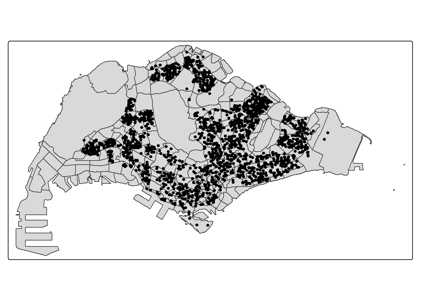
Notice that all the geospatial layers are within the same map extend. This shows that their referencing system and coordinate values are referred to similar spatial context. This is very important in any geospatial analysis.
Alternatively, we can also prepare an interactive point symbol map by using the code chunk below.
tmap_mode('view')
tm_shape(childcare_sf)+
tm_dots()tmap_mode('plot')
Note
Notice that at the interactive mode, tmap is using leaflet for R API. The advantage of this interactive pin map is it allows us to navigate and zoom around the map freely. We can also query the information of each simple feature (i.e. the point) by clicking of them. Last but not least, you can also change the background of the internet map layer. Currently, three internet map layers are provided. They are: ESRI.WorldGrayCanvas, OpenStreetMap, and ESRI.WorldTopoMap. The default is ESRI.WorldGrayCanvas.
Warning
Always remember to switch back to plot mode after the interactive map. This is because, each interactive mode will consume a connection. You should also avoid displaying ecessive numbers of interactive maps (i.e. not more than 10) in one RMarkdown document when publish on Netlify.
4.5 Geospatial Data wrangling
spatstat relies on its own specific data structures like ppp (planar point pattern) for point data and owin for observation windows. In this section, you will learn how to convert sf (Simple Features) objects into spatstat ppp and owin object.
4.5.1 Converting sf data frames to ppp class
spatstat requires the point event data in ppp object form. The code chunk below uses [as.ppp()] of spatstat package to convert childcare_sf to ppp format.
childcare_ppp <- as.ppp(childcare_sf)Next, class() of Base R will be used to verify the object class of childcare_ppp.
class(childcare_ppp)[1] "ppp"Great, it is in ppp object class!
You can take a quick look at the summary statistics of the newly converted ppp object by using the code chunk below.
summary(childcare_ppp)Marked planar point pattern: 1925 points
Average intensity 2.417323e-06 points per square unit
Coordinates are given to 11 decimal places
Mark variables: Name, Description
Summary:
Name Description
Length:1925 Length:1925
Class :character Class :character
Mode :character Mode :character
Window: rectangle = [11810.03, 45404.24] x [25596.33, 49300.88] units
(33590 x 23700 units)
Window area = 796335000 square units4.5.2 Creating owin object
When analysing spatial point patterns, it is a good practice to confine the analysis with a geographical area like Singapore boundary. In spatstat, an object called owin is specially designed to represent this polygonal region.
The code chunk below, as.owin() of spatstat is used to covert mpsz_sf into owin object of spatstat.
sg_owin <- as.owin(mpsz_cl)Again, class() will be used to verify the object class of sg_owin.
class(sg_owin)[1] "owin"The result above confirmed that sg_owin is indeed in owin object.
sg_owin object can be displayed by using plot() function.
plot(sg_owin)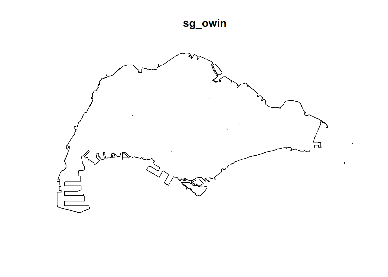
4.5.3 Combining point events object and owin object
In this last step of geospatial data wrangling, we will extract childcare events that are located within Singapore by using the code chunk below.
childcareSG_ppp = childcare_ppp[sg_owin]The output object combined both the point and polygon feature in one ppp object class as shown below.
childcareSG_pppMarked planar point pattern: 1925 points
Mark variables: Name, Description
window: polygonal boundary
enclosing rectangle: [2667.54, 55941.94] x [21448.47, 50256.33] units4.6 Clark-Evan Test for Nearest Neighbour Analysis
Nearest Neighbor Analysis (NNA) is a spatial statistics method that calculates the average distance between each point and its closest neighbor to determine if a pattern of points is clustered, dispersed, or randomly distributed.
Clark-Evans test is a specific statistical method used within NNA to quantify whether a point pattern is clustered, random, or uniformly spaced, using the Clark-Evans aggregation index (R) to describe this pattern. NNA provides a numerical value that describes the degree of clustering or regularity, and the Clark-Evans test calculates a specific index (R) for this purpose
Note
NNA is a broad term for methods that examine the spatial distribution of points, whereas the Clark-Evans test is a specific statistical method used within NNA to quantify whether a point pattern is clustered, random, or uniformly spaced, using the Clark-Evans aggregation index (R) to describe this pattern. NNA provides a numerical value that describes the degree of clustering or regularity, and the Clark-Evans test calculates a specific index (R) for this purpose.
In this section, we will perform the Clark-Evans test of aggregation for a spatial point pattern by using clarkevans.test() of spatstat.explore package.
The test hypotheses are:
Ho = The distribution of childcare services are randomly distributed.
H1= The distribution of childcare services are not randomly distributed.
The 95% confident interval will be used.
4.6.1 Perform the Clark-Evans test without CSR
clarkevans.test() of spatstat.explore package support two Clark-Evans test, namely: without CRS and with CRS. In the code chunk below, Clark-Evans test without CSR method is used.
clarkevans.test(childcareSG_ppp,
                correction="none",
                clipregion="sg_owin",
                alternative=c("clustered"))
    Clark-Evans test
    No edge correction
    Z-test

data:  childcareSG_ppp
R = 0.53532, p-value < 2.2e-16
alternative hypothesis: clustered (R < 1)
Quiz
- Draw statistical conclusion from the test result.
- Provide business communication from the statistical analysis.
4.6.2 Perform the Clark-Evans test with CSR
In the code chunk below, the argument method = “MonteCarlo” is used. In this case, the p-value for the test is computed by comparing the observed value of R to the results obtained from nsim (i.e. 39, 99, 999) simulated realisations of Complete Spatial Randomness conditional on the observed number of points.
clarkevans.test(childcareSG_ppp,
                correction="none",
                clipregion="sg_owin",
                alternative=c("clustered"),
                method="MonteCarlo",
                nsim=99)
    Clark-Evans test
    No edge correction
    Monte Carlo test based on 99 simulations of CSR with fixed n

data:  childcareSG_ppp
R = 0.53532, p-value = 0.01
alternative hypothesis: clustered (R < 1)
Quiz
- Draw statistical conclusion from the test result.
- Provide business communication from the statistical analysis.
4.7 Kernel Density Estimation Method
Kernel Density Estimation (KDE) is a valuable tool for visualising and analyzing first-order spatial point patterns. It is widely considered a method within Exploratory Spatial Data Analysis (ESDA) because it’s used to visualize and understand spatial data patterns by transforms discrete point data (like locations of childcare service, crime incidents or disease cases) into continuous density surfaces that reveal clusters and variations in event occurrences, without making prior assumptions about data distribution. It helps to begin understanding data distribution, identify hotspots, and explore relationships between spatial variables before performing more rigorous analysis.
In this section, you will learn how to compute the kernel density estimation (KDE) of childcare services in Singapore.
4.7.1 Working with automatic bandwidth selection method
The code chunk below computes a kernel density by using the following configurations of density() of spatstat:
- bw.diggle() automatic bandwidth selection method. Other recommended methods are bw.CvL(), bw.scott() or bw.ppl().
- The smoothing kernel used is gaussian, which is the default. Other smoothing methods are: “epanechnikov”, “quartic” or “disc”.
- The intensity estimate is corrected for edge effect bias by using method described by Jones (1993) and Diggle (2010, equation 18.9). The default is FALSE.
kde_SG_diggle <- density(
  childcareSG_ppp,
  sigma=bw.diggle,
  edge=TRUE,
  kernel="gaussian")
Note
The output of density() of spatstat is an im class, represents a two-dimensional pixel image. It’s a class used to store and manipulate raster data, where the spatial domain is divided into a grid of rectangular pixels. Each pixel has an associated value, which can be numerical or a factor.
The plot() function of Base R is then used to display the kernel density derived.
plot(kde_SG_diggle)
In the code chunk below, summary() of Base R is used to print the summary report of the
summary(kde_SG_diggle)real-valued pixel image
128 x 128 pixel array (ny, nx)
enclosing rectangle: [2667.538, 55941.94] x [21448.47, 50256.33] units
dimensions of each pixel: 416 x 225.0614 units
Image is defined on a subset of the rectangular grid
Subset area = 669941961.12249 square units
Subset area fraction = 0.437
Pixel values (inside window):
range = [-6.584123e-21, 3.063698e-05]
integral = 1927.788
mean = 2.877545e-06
Warning
The density values of the output range from 0 to 0.00003727443 which is way too small to comprehend. This is because the default unit of measurement of svy21 is in meter. As a result, the density values computed is in “number of points per square meter”.
Before we move on to next section, it is good to know that you can retrieve the bandwidth used to compute the kde layer by using the code chunk below.
bw <- bw.diggle(childcareSG_ppp)
bw
sigma
295.9712 4.7.2 Rescalling KDE values
In the code chunk below, rescale.ppp() is used to covert the unit of measurement from meter to kilometer.
childcareSG_ppp_km <- rescale.ppp(
  childcareSG_ppp, 1000, "km")
Now, we can re-run density() using the resale data set and plot the output kde map.
kde_childcareSG_km <- density(childcareSG_ppp_km,
                              sigma=bw.diggle,
                              edge=TRUE,
                              kernel="gaussian")
Next, plot() is used to plot the kde object as shown below.
plot(kde_childcareSG_km)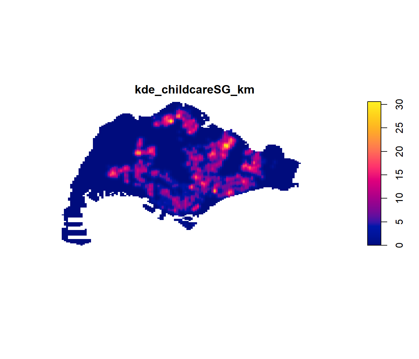
Notice that output image looks identical to the earlier version, the only changes in the data values (refer to the legend).
4.7.3 Working with different automatic badwidth methods
Beside bw.diggle(), there are three other spatstat functions can be used to determine the bandwidth, they are: bw.CvL(), bw.scott(), and bw.ppl().
Let us take a look at the bandwidth return by these automatic bandwidth calculation methods by using the code chunk below.
bw.CvL(childcareSG_ppp_km) sigma
4.357209 bw.scott(childcareSG_ppp_km) sigma.x sigma.y
2.159749 1.396455 bw.ppl(childcareSG_ppp_km) sigma
0.378997 bw.diggle(childcareSG_ppp_km) sigma
0.2959712 Baddeley et. (2016) suggested the use of the bw.ppl() algorithm because past experience shown that it tends to produce the more appropriate values when the pattern consists predominantly of tight clusters. But they also insist that if the purpose of once study is to detect a single tight cluster in the midst of random noise then the bw.diggle() method seems to work best.
The code chunk beow will be used to compare the output of using bw.diggle and bw.ppl methods.
kde_childcareSG.ppl <- density(childcareSG_ppp_km,
                               sigma=bw.ppl,
                               edge=TRUE,
                               kernel="gaussian")
par(mfrow=c(1,2))
plot(kde_childcareSG_km, main = "bw.diggle")
plot(kde_childcareSG.ppl, main = "bw.ppl")
4.7.4 Working with different kernel methods
By default, the kernel method used in density.ppp() is gaussian. But there are three other options, namely: Epanechnikov, Quartic and Dics.
The code chunk below will be used to compute three more kernel density estimations by using these three kernel function.
par(mfrow=c(2,2))
plot(density(childcareSG_ppp_km,
             sigma=0.2959712,
             edge=TRUE,
             kernel="gaussian"),
     main="Gaussian")
plot(density(childcareSG_ppp_km,
             sigma=0.2959712,
             edge=TRUE,
             kernel="epanechnikov"),
     main="Epanechnikov")
plot(density(childcareSG_ppp_km,
             sigma=0.2959712,
             edge=TRUE,
             kernel="quartic"),
     main="Quartic")
plot(density(childcareSG_ppp_km,
             sigma=0.2959712,
             edge=TRUE,
             kernel="disc"),
     main="Disc")
4.8 Fixed and Adaptive KDE
4.8.1 Computing KDE by using fixed bandwidth
Next, you will compute a KDE layer by defining a bandwidth of 600 meter. Notice that in the code chunk below, the sigma value used is 0.6. This is because the unit of measurement of childcareSG_ppp_km object is in kilometer, hence the 600m is 0.6km.
kde_childcareSG_fb <- density(childcareSG_ppp_km,
                              sigma=0.6,
                              edge=TRUE,
                              kernel="gaussian")
plot(kde_childcareSG_fb)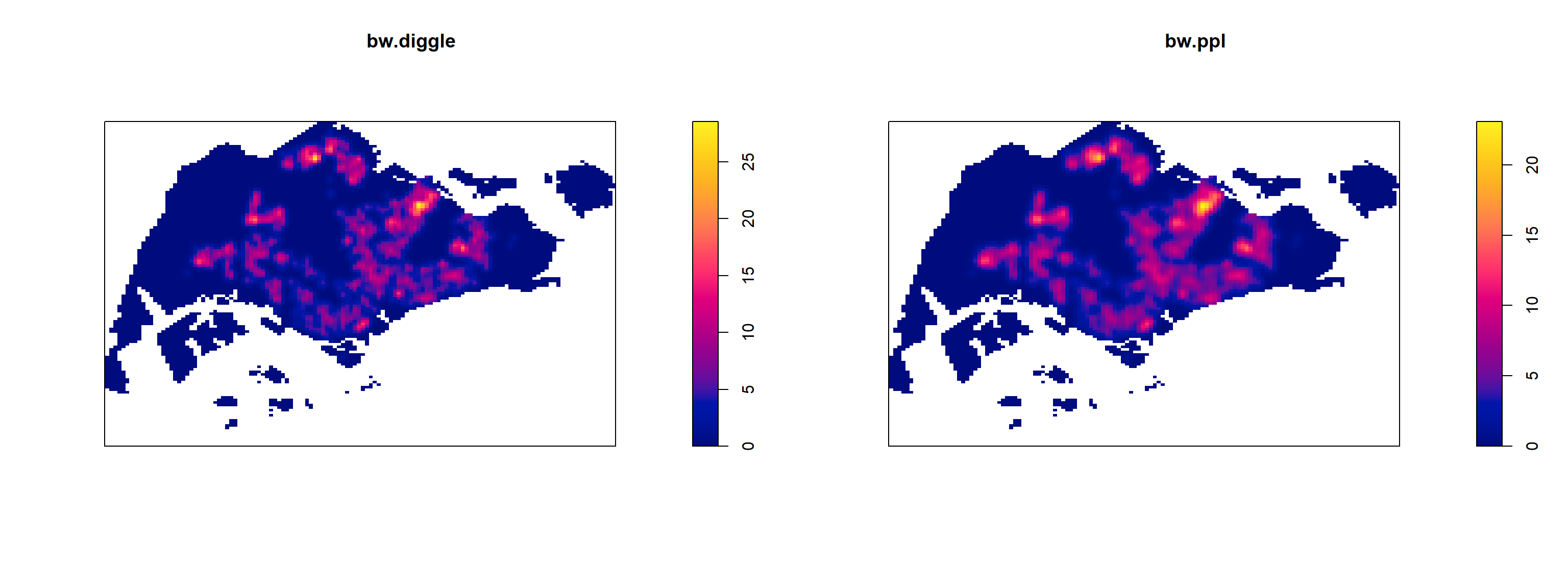
4.8.2 Computing KDE by using adaptive bandwidth
Fixed bandwidth method is very sensitive to highly skew distribution of spatial point patterns over geographical units for example urban versus rural. One way to overcome this problem is by using adaptive bandwidth instead.
In this section, you will learn how to derive adaptive kernel density estimation by using density.adaptive() of spatstat.
kde_childcareSG_ab <- adaptive.density(
  childcareSG_ppp_km,
  method="kernel")
plot(kde_childcareSG_ab)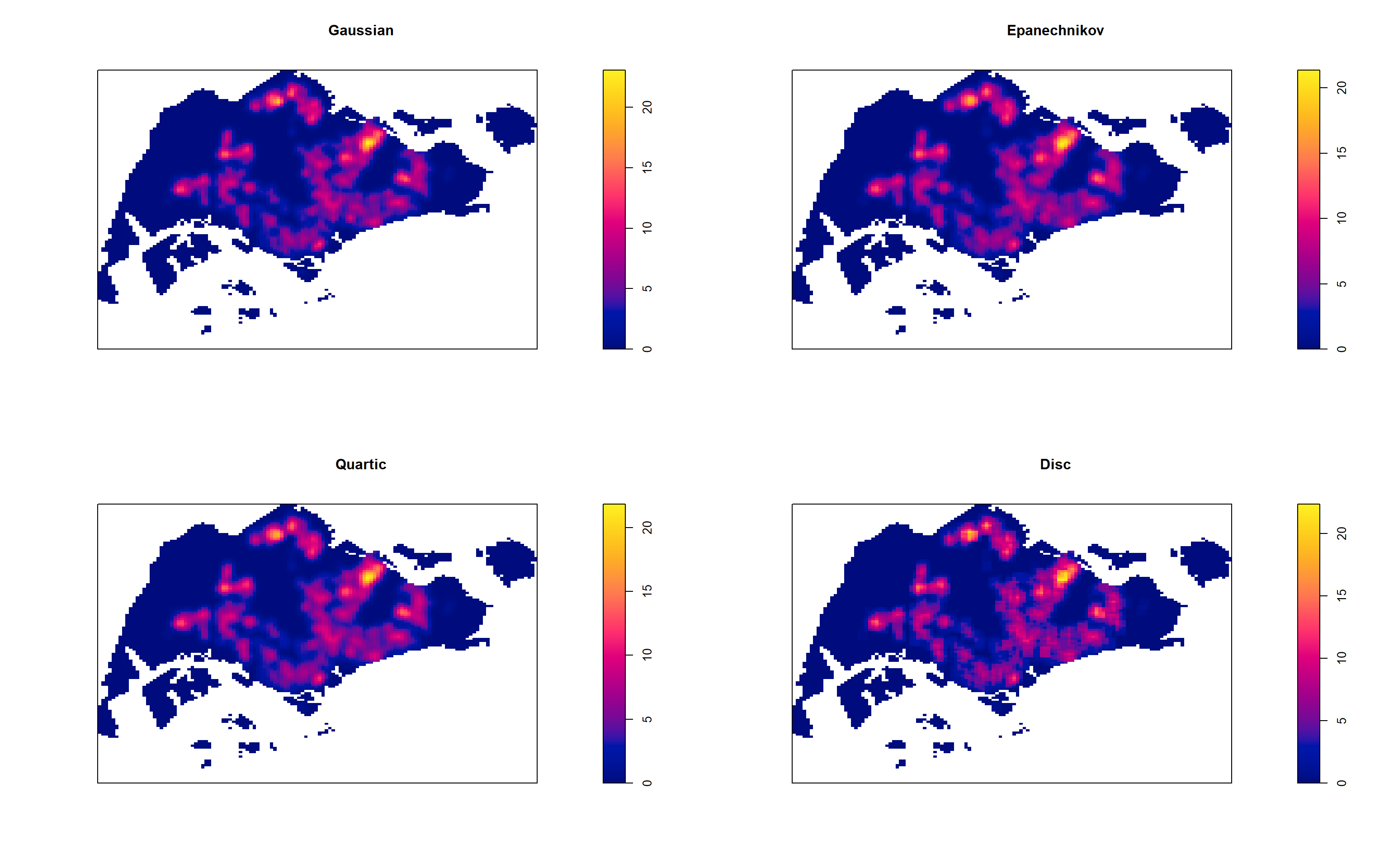
We can compare the fixed and adaptive kernel density estimation outputs by using the code chunk below.
par(mfrow=c(1,2))
plot(kde_childcareSG_fb, main = "Fixed bandwidth")
plot(kde_childcareSG_ab, main = "Adaptive bandwidth")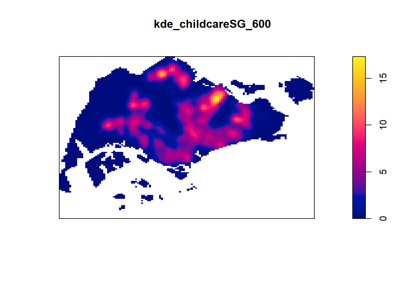
4.9 Plotting cartographic quality KDE map
4.9.1 Converting gridded output into raster
Next, we will convert the im kernal density objects into SpatRaster object by using rast() of terra package.
kde_childcareSG_bw_terra <- rast(kde_childcareSG_km)Again, class() is used to verify if kde_childcareSG_bw_terra data are belong to SpatRaster class.
class(kde_childcareSG_bw_terra)[1] "SpatRaster"
attr(,"package")
[1] "terra"Yes, it is indeed in SpatRaster class.
Let us take a look at the properties of kde_childcareSG_bw_terra .
kde_childcareSG_bw_terraclass : SpatRaster
size : 128, 128, 1 (nrow, ncol, nlyr)
resolution : 0.4162063, 0.2250614 (x, y)
extent : 2.667538, 55.94194, 21.44847, 50.25633 (xmin, xmax, ymin, ymax)
coord. ref. :
source(s) : memory
name : lyr.1
min value : -5.824417e-15
max value : 3.063698e+01
unit : km Notice that the crs property is empty.
4.9.2 Assigning projection systems
In code chunk below, crs() of terra is used to assign the CRS information on kde_childcareSG_bw_terra layer.
crs(kde_childcareSG_bw_terra) <- "EPSG:3414"Let us take a look at the properties of kde_childcareSG_bw_raster RasterLayer.
kde_childcareSG_bw_terraclass : SpatRaster
size : 128, 128, 1 (nrow, ncol, nlyr)
resolution : 0.4162063, 0.2250614 (x, y)
extent : 2.667538, 55.94194, 21.44847, 50.25633 (xmin, xmax, ymin, ymax)
coord. ref. : SVY21 / Singapore TM (EPSG:3414)
source(s) : memory
name : lyr.1
min value : -5.824417e-15
max value : 3.063698e+01
unit : km Notice that the coordicates reference (i.e. coord. ref.) is in SVY21 now.
4.9.3 Plotting KDE map with tmap
Finally, we will display the raster in cartographic quality map using tmap package.
tm_shape(kde_childcareSG_bw_terra) +
  tm_raster(col.scale =
              tm_scale_continuous(
                values = "viridis"),
            col.legend = tm_legend(
            title = "Density values",
            title.size = 0.7,
            text.size = 0.7,
            bg.color = "white",
            bg.alpha = 0.7,
            position = tm_pos_in(
              "right", "bottom"),
            frame = TRUE)) +
  tm_graticules(labels.size = 0.7) +
  tm_compass() +
  tm_layout(scale = 1.0)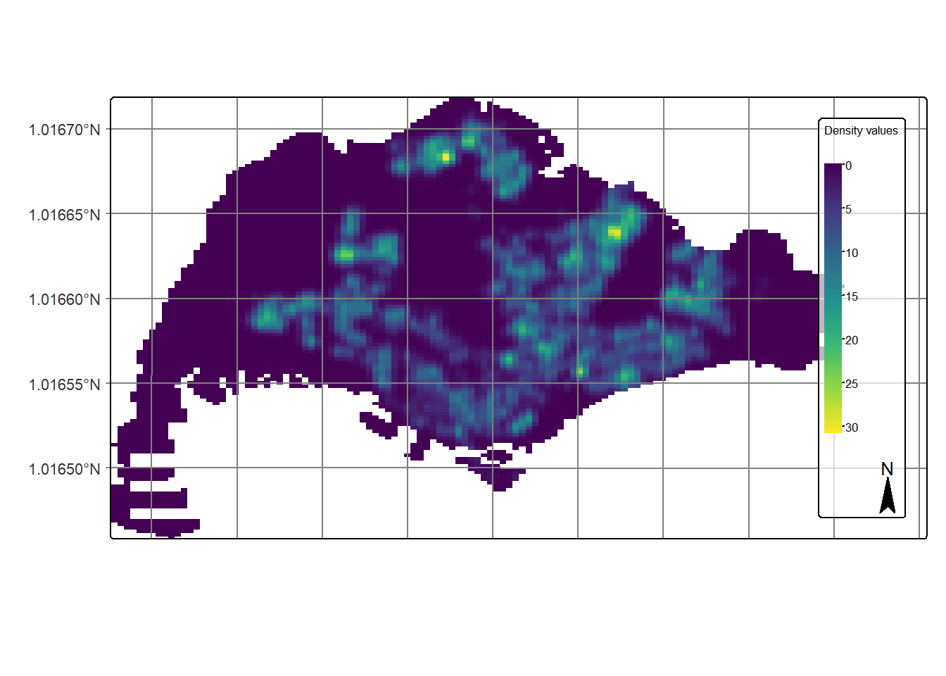
Notice that the raster values are encoded explicitly onto the raster pixel using the values in “layer.1” field.
4.10 First Order SPPA at the Planning Subzone Level
In this section, we would like to further our analysis at the planning area level. For simplicity reason, we will focus on Punggol, Tampines Chua Chu Kand and Jurong West planning areas
4.10.1 Geospatial data wrangling
4.10.1.1 Extracting study area
The code chunk below will be used to extract the target planning areas.
pg <- mpsz_cl %>%
  filter(PLN_AREA_N == "PUNGGOL")
tm <- mpsz_cl %>%
  filter(PLN_AREA_N == "TAMPINES")
ck <- mpsz_cl %>%
  filter(PLN_AREA_N == "CHOA CHU KANG")
jw <- mpsz_cl %>%
  filter(PLN_AREA_N == "JURONG WEST")
It is always a good practice to review the extracted areas. The code chunk below will be used to plot the extracted planning areas.
par(mfrow=c(2,2))
plot(st_geometry(pg), main = "Ponggol")
plot(st_geometry(tm), main = "Tampines")
plot(st_geometry(ck), main = "Choa Chu Kang")
plot(st_geometry(jw), main = "Jurong West")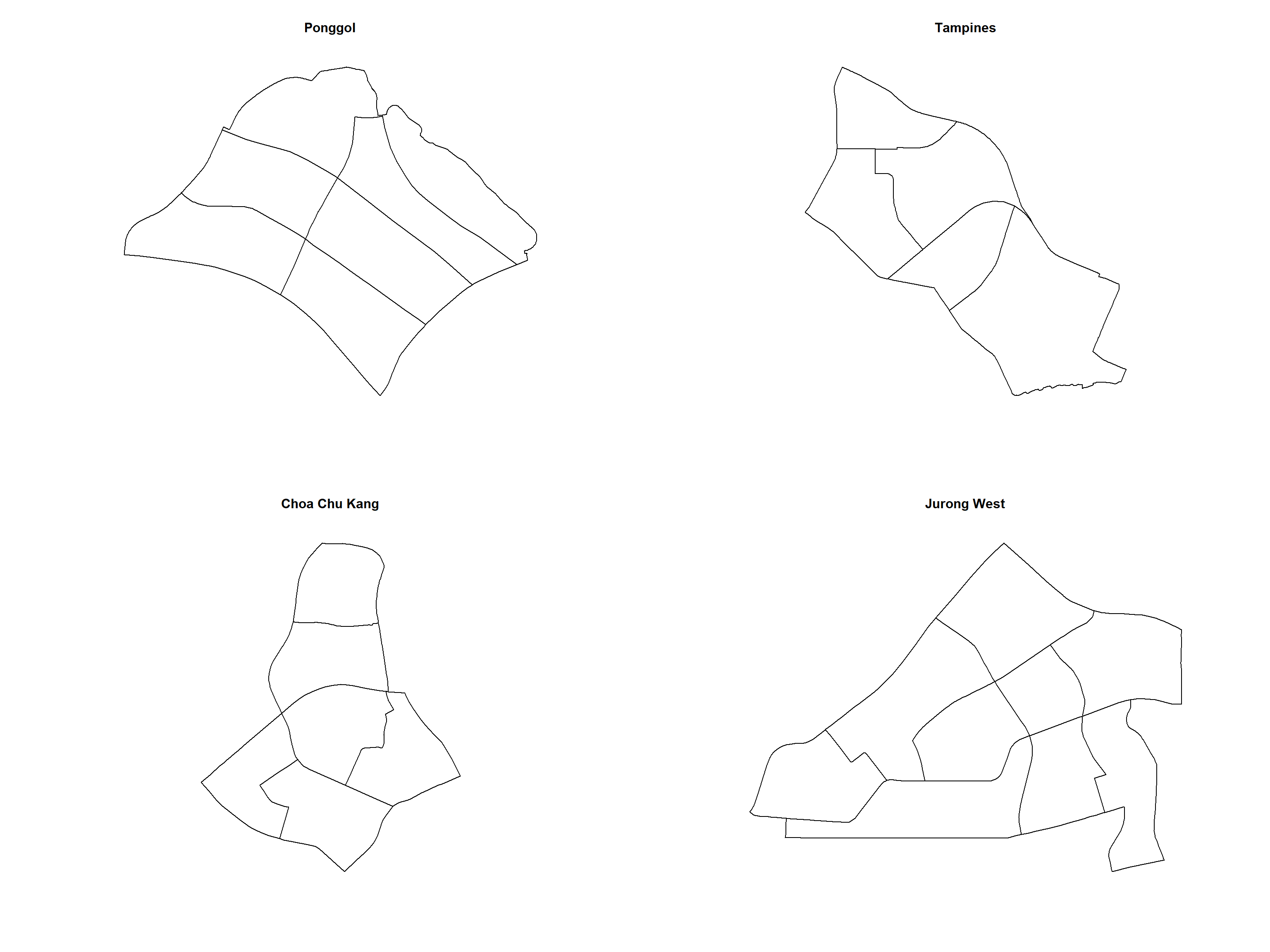
4.10.1.2 Creating owin object
Now, we will convert these sf objects into owin objects that is required by spatstat.
pg_owin = as.owin(pg)
tm_owin = as.owin(tm)
ck_owin = as.owin(ck)
jw_owin = as.owin(jw)
4.10.1.3 Combining point events object and owin object
childcare_pg_ppp = childcare_ppp[pg_owin]
childcare_tm_ppp = childcare_ppp[tm_owin]
childcare_ck_ppp = childcare_ppp[ck_owin]
childcare_jw_ppp = childcare_ppp[jw_owin]
Next, rescale.ppp() function is used to trasnform the unit of measurement from metre to kilometre.
childcare_pg_ppp.km = rescale.ppp(childcare_pg_ppp, 1000, "km")
childcare_tm_ppp.km = rescale.ppp(childcare_tm_ppp, 1000, "km")
childcare_ck_ppp.km = rescale.ppp(childcare_ck_ppp, 1000, "km")
childcare_jw_ppp.km = rescale.ppp(childcare_jw_ppp, 1000, "km")
The code chunk below is used to plot these four study areas and the locations of the childcare centres.
par(mfrow=c(2,2))
plot(unmark(childcare_pg_ppp.km),
  main="Punggol")
plot(unmark(childcare_tm_ppp.km),
  main="Tampines")
plot(unmark(childcare_ck_ppp.km),
  main="Choa Chu Kang")
plot(unmark(childcare_jw_ppp.km),
  main="Jurong West")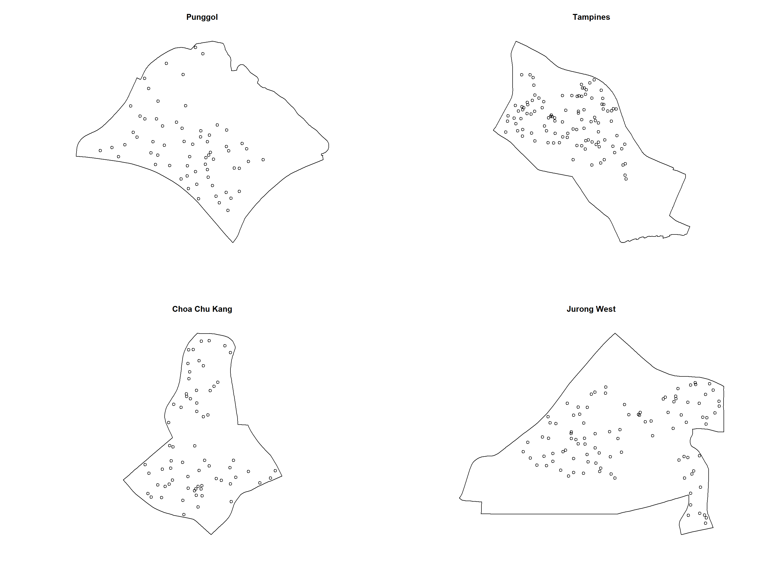
4.10.2 Clark and Evans Test
4.10.2.1 Choa Chu Kang planning area
In the code chunk below, clarkevans.test() of spatstat is used to performs Clark-Evans test of aggregation for childcare centre in Choa Chu Kang planning area.
clarkevans.test(childcare_ck_ppp,
                correction="none",
                clipregion=NULL,
                alternative=c("two.sided"),
                nsim=999)
    Clark-Evans test
    No edge correction
    Z-test

data:  childcare_ck_ppp
R = 0.84097, p-value = 0.008866
alternative hypothesis: two-sided
4.10.2.2 Tampines planning area
In the code chunk below, the similar test is used to analyse the spatial point patterns of childcare centre in Tampines planning area.
clarkevans.test(childcare_tm_ppp,
                correction="none",
                clipregion=NULL,
                alternative=c("two.sided"),
                nsim=999)
    Clark-Evans test
    No edge correction
    Z-test

data:  childcare_tm_ppp
R = 0.66817, p-value = 6.58e-12
alternative hypothesis: two-sided
4.10.3 Computing KDE surfaces by planning area
The code chunk below will be used to compute the KDE of these four planning area. bw.diggle method is used to derive the bandwidth of each
par(mfrow=c(2,2))
plot(density(childcare_pg_ppp.km,
             sigma=bw.diggle,
             edge=TRUE,
             kernel="gaussian"),
     main="Punggol")
plot(density(childcare_tm_ppp.km,
             sigma=bw.diggle,
             edge=TRUE,
             kernel="gaussian"),
     main="Tempines")
plot(density(childcare_ck_ppp.km,
             sigma=bw.diggle,
             edge=TRUE,
             kernel="gaussian"),
     main="Choa Chu Kang")
plot(density(childcare_jw_ppp.km,
             sigma=bw.diggle,
             edge=TRUE,
             kernel="gaussian"),
     main="Jurong West")