pacman::p_load(sf, spNetwork, tmap, tidyverse)7 Network Constrained Spatial Point Patterns Analysis
7.1 Overview
Network constrained Spatial Point Patterns Analysis (NetSPAA) is a collection of spatial point patterns analysis methods special developed for analysing spatial point event occurs on or alongside network. The spatial point event can be locations of traffic accident or childcare centre for example. The network, on the other hand can be a road network or river network.
In this hands-on exercise, you are going to gain hands-on experience on using appropriate functions of spNetwork package:
- to derive network kernel density estimation (NKDE), and
- to perform network G-function and k-function analysis
7.2 The Data
In this study, we will analyse the spatial distribution of childcare centre in Punggol planning area. For the purpose of this study, two geospatial data sets will be used. They are:
- Punggol_St, a line features geospatial data which store the road network within Punggol Planning Area.
- Punggol_CC, a point feature geospatial data which store the location of childcare centres within Punggol Planning Area.
Both data sets are in ESRI shapefile format.
7.3 Installing and launching the R packages
In this hands-on exercise, four R packages will be used, they are:
- spNetwork, which provides functions to perform Spatial Point Patterns Analysis such as kernel density estimation (KDE) and K-function on network. It also can be used to build spatial matrices (‘listw’ objects like in ‘spdep’ package) to conduct any kind of traditional spatial analysis with spatial weights based on reticular distances.
- sf package provides functions to manage, processing, and manipulate Simple Features, a formal geospatial data standard that specifies a storage and access model of spatial geometries such as points, lines, and polygons.
- tmap which provides functions for plotting cartographic quality static point patterns maps or interactive maps by using leaflet API.
Use the code chunk below to install and launch the four R packages.
7.4 Data Import and Preparation
The code chunk below uses st_read() of sf package to important Punggol_St and Punggol_CC geospatial data sets into RStudio as sf data frames.
network <- st_read(dsn="chap07/data/geospatial",
                   layer="Punggol_St")
Reading layer `Punggol_St' from data source
`C:\tskam\r4gdsa\chap07\data\geospatial' using driver `ESRI Shapefile'
Simple feature collection with 2642 features and 2 fields
Geometry type: LINESTRING
Dimension: XY
Bounding box: xmin: 34038.56 ymin: 40941.11 xmax: 38882.85 ymax: 44801.27
Projected CRS: SVY21 / Singapore TMchildcare <- st_read(dsn="chap07/data/geospatial",
layer="Punggol_CC")Reading layer `Punggol_CC' from data source
`C:\tskam\r4gdsa\chap07\data\geospatial' using driver `ESRI Shapefile'
Simple feature collection with 61 features and 1 field
Geometry type: POINT
Dimension: XYZ
Bounding box: xmin: 34423.98 ymin: 41503.6 xmax: 37619.47 ymax: 44685.77
z_range: zmin: 0 zmax: 0
Projected CRS: SVY21 / Singapore TMWe can examine the structure of the output simple features data tables in RStudio. Alternative, code chunk below can be used to print the content of network and childcare simple features objects by using the code chunk below.
childcareSimple feature collection with 61 features and 1 field
Geometry type: POINT
Dimension: XYZ
Bounding box: xmin: 34423.98 ymin: 41503.6 xmax: 37619.47 ymax: 44685.77
z_range: zmin: 0 zmax: 0
Projected CRS: SVY21 / Singapore TM
First 10 features:
Name geometry
1 kml_10 POINT Z (36173.81 42550.33 0)
2 kml_99 POINT Z (36479.56 42405.21 0)
3 kml_100 POINT Z (36618.72 41989.13 0)
4 kml_101 POINT Z (36285.37 42261.42 0)
5 kml_122 POINT Z (35414.54 42625.1 0)
6 kml_161 POINT Z (36545.16 42580.09 0)
7 kml_172 POINT Z (35289.44 44083.57 0)
8 kml_188 POINT Z (36520.56 42844.74 0)
9 kml_205 POINT Z (36924.01 41503.6 0)
10 kml_222 POINT Z (37141.76 42326.36 0)networkSimple feature collection with 2642 features and 2 fields
Geometry type: LINESTRING
Dimension: XY
Bounding box: xmin: 34038.56 ymin: 40941.11 xmax: 38882.85 ymax: 44801.27
Projected CRS: SVY21 / Singapore TM
First 10 features:
LINK_ID ST_NAME geometry
1 116130894 PUNGGOL RD LINESTRING (36546.89 44574....
2 116130897 PONGGOL TWENTY-FOURTH AVE LINESTRING (36546.89 44574....
3 116130901 PONGGOL SEVENTEENTH AVE LINESTRING (36012.73 44154....
4 116130902 PONGGOL SEVENTEENTH AVE LINESTRING (36062.81 44197....
5 116130907 PUNGGOL CENTRAL LINESTRING (36131.85 42755....
6 116130908 PUNGGOL RD LINESTRING (36112.93 42752....
7 116130909 PUNGGOL CENTRAL LINESTRING (36127.4 42744.5...
8 116130910 PUNGGOL FLD LINESTRING (35994.98 42428....
9 116130911 PUNGGOL FLD LINESTRING (35984.97 42407....
10 116130912 EDGEFIELD PLNS LINESTRING (36200.87 42219....When I exploring spNetwork’s functions, it came to my attention that spNetwork is expecting the geospatial data contains complete CRS information.
7.5 Visualising the Geospatial Data
Before we jump into the analysis, it is a good practice to visualise the geospatial data. There are at least two ways to visualise the geospatial data. One way is by using plot() of Base R as shown in the code chunk below.
plot(st_geometry(network))
plot(childcare,add=T,col='red',pch = 19)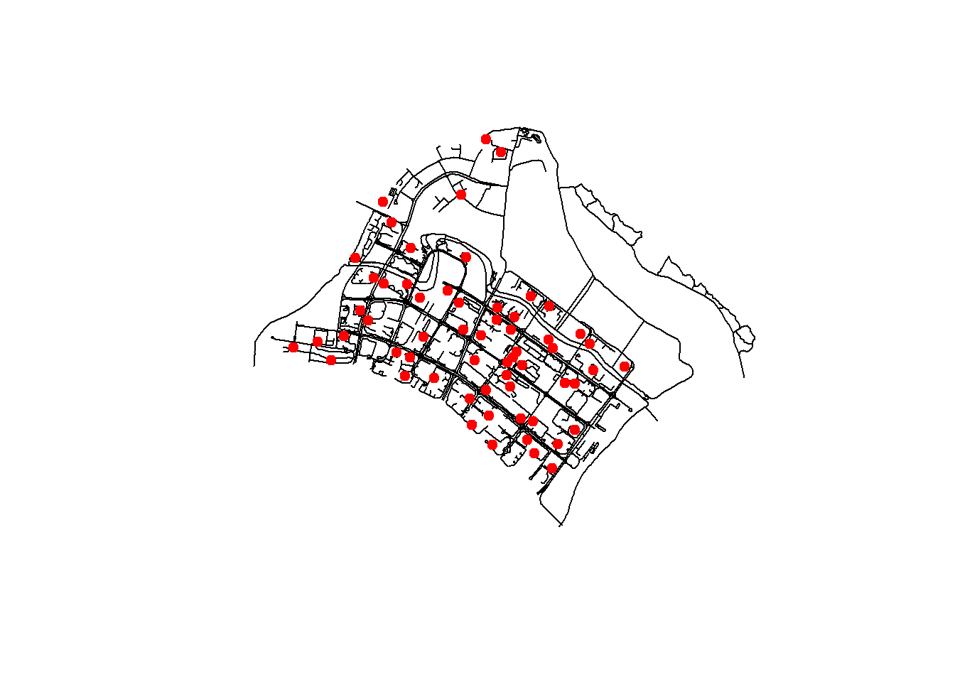
To visualise the geospatial data with high cartographic quality and interactive manner, the mapping function of tmap package can be used as shown in the code chunk below.
tmap_mode('view')
tm_shape(childcare) +
  tm_dots() +
  tm_shape(network) +
tm_lines()tmap_mode('plot')7.6 Network KDE (NKDE) Analysis
In this section, we will perform NKDE analysis by using appropriate functions provided in spNetwork package.
7.6.1 Preparing the lixels objects
Before computing NKDE, the SpatialLines object need to be cut into lixels with a specified minimal distance. This task can be performed by using with lixelize_lines() of spNetwork as shown in the code chunk below.
lixels <- lixelize_lines(network,
                         700,
                         mindist = 375)
What can we learned from the code chunk above:
- The length of a lixel, lx_length is set to 700m, and
- The minimum length of a lixel, mindist is set to 350m.
After cut, if the length of the final lixel is shorter than the minimum distance, then it is added to the previous lixel. If NULL, then mindist = maxdist/10. Also note that the segments that are already shorter than the minimum distance are not modified
Note: There is another function called lixelize_lines.mc() which provide multicore support.
7.6.2 Generating line centre points
Next, lines_center() of spNetwork will be used to generate a SpatialPointsDataFrame (i.e. samples) with line centre points as shown in the code chunk below.
samples <- lines_center(lixels) The points are located at center of the line based on the length of the line.
7.6.3 Performing NKDE
We are ready to computer the NKDE by using the code chunk below.
densities <- nkde(network,
                  events = childcare,
                  w = rep(1, nrow(childcare)),
                  samples = samples,
                  kernel_name = "quartic",
                  bw = 300,
                  div= "bw",
                  method = "simple",
                  digits = 1,
                  tol = 1,
                  grid_shape = c(1,1),
                  max_depth = 8,
                  agg = 5,
                  sparse = TRUE,
                  verbose = FALSE)
What can we learn from the code chunk above?
- kernel_name argument indicates that quartic kernel is used. Are possible kernel methods supported by spNetwork are: triangle, gaussian, scaled gaussian, tricube, cosine ,triweight, epanechnikov or uniform.
- method argument indicates that simple method is used to calculate the NKDE. Currently, spNetwork support three popular methods, they are:
- method=“simple”. This first method was presented by Xie et al. (2008) and proposes an intuitive solution. The distances between events and sampling points are replaced by network distances, and the formula of the kernel is adapted to calculate the density over a linear unit instead of an areal unit.
- method=“discontinuous”. The method is proposed by Okabe et al (2008), which equally “divides” the mass density of an event at intersections of lixels.
- method=“continuous”. If the discontinuous method is unbiased, it leads to a discontinuous kernel function which is a bit counter-intuitive. Okabe et al (2008) proposed another version of the kernel, that divide the mass of the density at intersection but adjusts the density before the intersection to make the function continuous.
The user guide of spNetwork package provide a comprehensive discussion of nkde(). You should read them at least once to have a basic understanding of the various parameters that can be used to calibrate the NKDE model.
7.6.3.1 Visualising NKDE
Before we can visualise the NKDE values, code chunk below will be used to insert the computed density values (i.e. densities) into samples and lixels objects as density field.
samples$density <- densities
lixels$density <- densities
Since svy21 projection system is in meter, the computed density values are very small i.e. 0.0000005. The code chunk below is used to resale the density values from number of events per meter to number of events per kilometer.
# rescaling to help the mapping
samples$density <- samples$density*1000
lixels$density <- lixels$density*1000
The code below uses appropriate functions of tmap package to prepare interactive and high cartographic quality map visualisation.
tmap_mode('view')
tm_shape(lixels)+
  tm_lines(col="density")+
tm_shape(childcare)+
  tm_dots()
tmap_mode('plot')
The interactive map above effectively reveals road segments (darker color) with relatively higher density of childcare centres than road segments with relatively lower density of childcare centres (lighter color)
7.7 Network Constrained G- and K-Function Analysis
In this section, we are going to perform complete spatial randomness (CSR) test by using kfunctions() of spNetwork package. The null hypothesis is defined as:
Ho: The observed spatial point events (i.e distribution of childcare centres) are uniformly distributed over a street network in Punggol Planning Area.
The CSR test is based on the assumption of the binomial point process which implies the hypothesis that the childcare centres are randomly and independently distributed over the street network.
If this hypothesis is rejected, we may infer that the distribution of childcare centres are spatially interacting and dependent on each other; as a result, they may form nonrandom patterns.
kfun_childcare <- kfunctions(network,
                             childcare,
                             start = 0,
                             end = 1000,
                             step = 50,
                             width = 50,
                             nsim = 50,
                             resolution = 50,
                             verbose = FALSE,
                             conf_int = 0.05)
What can we learn from the code chunk above?
There are ten arguments used in the code chunk above they are:
- lines: A SpatialLinesDataFrame with the sampling points. The geometries must be a SpatialLinesDataFrame (may crash if some geometries are invalid).
- points: A SpatialPointsDataFrame representing the points on the network. These points will be snapped on the network.
- start: A double, the start value for evaluating the k and g functions.
- end: A double, the last value for evaluating the k and g functions.
- step: A double, the jump between two evaluations of the k and g function.
- width: The width of each donut for the g-function.
- nsim: An integer indicating the number of Monte Carlo simulations required. In the above example, 50 simulation was performed. Note: most of the time, more simulations are required for inference
- resolution: When simulating random points on the network, selecting a resolution will reduce greatly the calculation time. When resolution is null the random points can occur everywhere on the graph. If a value is specified, the edges are split according to this value and the random points are selected vertices on the new network.
- conf_int: A double indicating the width confidence interval (default = 0.05).
For the usage of other arguments, you should refer to the user guide of spNetwork package.
The output of kfunctions() is a list with the following values:
- plotkA, a ggplot2 object representing the values of the k-function
- plotgA, a ggplot2 object representing the values of the g-function
- valuesA, a DataFrame with the values used to build the plots
For example, we can visualise the ggplot2 object of k-function by using the code chunk below.
kfun_childcare$plotk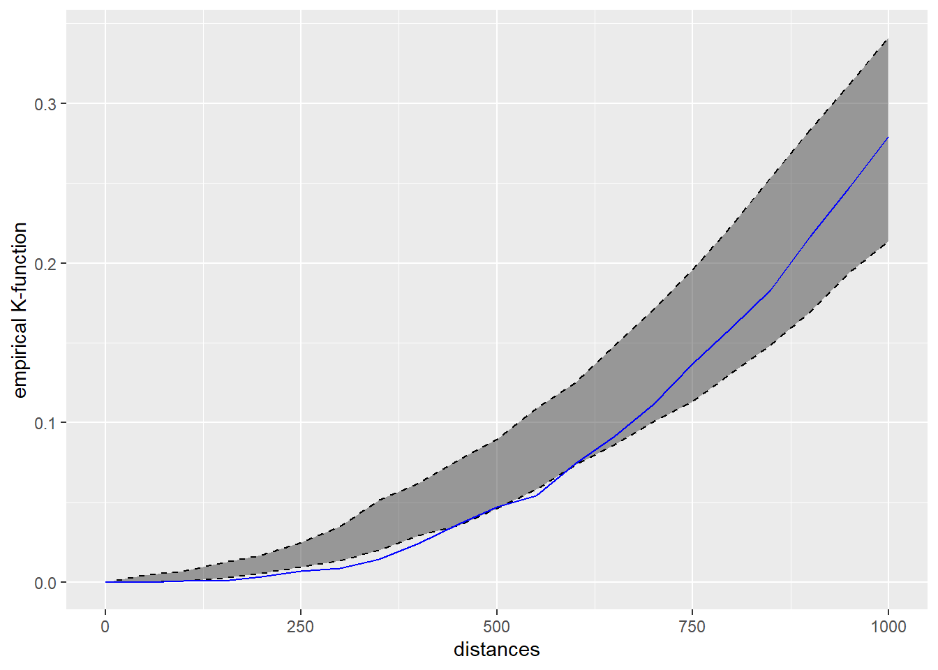
The blue line is the empirical network K-function of the childcare centres in Punggol planning area. The gray envelop represents the results of the 50 simulations in the interval 2.5% - 97.5%. Because the blue line between the distance of 250m-400m are below the gray area, we can infer that the childcare centres in Punggol planning area resemble regular pattern at the distance of 250m-400m.