pacman::p_load(tmap, sf, DT, stplanr, tidyverse)15 Processing and Visualising Flow Data
15.1 Overview
Spatial interaction represent the flow of people, material, or information between locations in geographical space. It encompasses everything from freight shipments, energy flows, and the global trade in rare antiquities, to flight schedules, rush hour woes, and pedestrian foot traffic.
Each spatial interaction, as an analogy for a set of movements, is composed of a discrete origin/destination pair. Each pair can be represented as a cell in a matrix where rows are related to the locations (centroids) of origin, while columns are related to locations (centroids) of destination. Such a matrix is commonly known as an origin/destination matrix, or a spatial interaction matrix.
In this hands-on exercise, you will learn how to build an OD matrix by using Passenger Volume by Origin Destination Bus Stops data set downloaded from LTA DataMall. By the end of this hands-on exercise, you will be able:
- to import and extract OD data for a selected time interval,
- to import and save geospatial data (i.e. bus stops and mpsz) into sf tibble data frame objects,
- to populate planning subzone code into bus stops sf tibble data frame,
- to construct desire lines geospatial data from the OD data, and
- to visualise passenger volume by origin and destination bus stops by using the desire lines data.
15.2 Getting Started
For the purpose of this exercise, five r packages will be used. They are:
- sf for importing, integrating, processing and transforming geospatial data.
- tidyverse for importing, integrating, wrangling and visualising data.
- tmap for creating elegent and cartographic quality thematic maps.
- stplanr provides functions for solving common problems in transport planning and modelling such as downloading and cleaning transport datasets; creating geographic “desire lines” from origin-destination (OD) data; route assignment, locally and interfaces to routing services such as CycleStreets.net; calculation of route segment attributes such as bearing and aggregate flow; and ‘travel watershed’ analysis.
- DT provides an R interface to the JavaScript library DataTables. R data objects (matrices or data frames) can be displayed as tables on HTML pages, and DataTables provides filtering, pagination, sorting, and many other features in the tables.
15.3 Preparing the Flow Data
15.3.1 Importing the OD data
Firstly, we will import the Passenger Volume by Origin Destination Bus Stops data set downloaded from LTA DataMall by using read_csv() of readr package.
odbus <- read_csv("chap15/data/aspatial/origin_destination_bus_202210.csv")Let use display the odbus tibble data table by using the code chunk below.
glimpse(odbus)Rows: 5,122,925
Columns: 7
$ YEAR_MONTH <chr> "2022-10", "2022-10", "2022-10", "2022-10", "2022-…
$ DAY_TYPE <chr> "WEEKDAY", "WEEKENDS/HOLIDAY", "WEEKENDS/HOLIDAY",…
$ TIME_PER_HOUR <dbl> 10, 10, 7, 11, 16, 16, 20, 7, 7, 11, 11, 8, 11, 11…
$ PT_TYPE <chr> "BUS", "BUS", "BUS", "BUS", "BUS", "BUS", "BUS", "…
$ ORIGIN_PT_CODE <dbl> 65239, 65239, 23519, 52509, 54349, 54349, 43371, 8…
$ DESTINATION_PT_CODE <dbl> 65159, 65159, 23311, 42041, 53241, 53241, 14139, 9…
$ TOTAL_TRIPS <dbl> 2, 1, 2, 1, 1, 4, 1, 3, 1, 5, 2, 5, 15, 40, 1, 1, …A quick check of odbus tibble data frame shows that the values in OROGIN_PT_CODE and DESTINATON_PT_CODE are in numeric data type. Hence, the code chunk below is used to convert these data values into character data type.
odbus$ORIGIN_PT_CODE <- as.factor(odbus$ORIGIN_PT_CODE)
odbus$DESTINATION_PT_CODE <- as.factor(odbus$DESTINATION_PT_CODE) 15.3.2 Extracting the study data
For the purpose of this exercise, we will extract commuting flows on weekday and between 6 and 9 o’clock.
odbus6_9 <- odbus %>%
filter(DAY_TYPE == "WEEKDAY") %>%
filter(TIME_PER_HOUR >= 6 &
TIME_PER_HOUR <= 9) %>%
group_by(ORIGIN_PT_CODE,
DESTINATION_PT_CODE) %>%
summarise(TRIPS = sum(TOTAL_TRIPS))Table below shows the content of odbus6_9
datatable(odbus6_9)We will save the output in rds format for future used.
write_rds(odbus6_9, "chap15/data/rds/odbus6_9.rds")The code chunk below will be used to import the save odbus6_9.rds into R environment.
odbus6_9 <- read_rds("chap15/data/rds/odbus6_9.rds")15.4 Working with Geospatial Data
For the purpose of this exercise, two geospatial data will be used. They are:
- BusStop: This data provides the location of bus stop as at last quarter of 2022.
- MPSZ-2019: This data provides the sub-zone boundary of URA Master Plan 2019.
Both data sets are in ESRI shapefile format.
15.4.1 Importing geospatial data
Two geospatial data will be used in this exercise, they are:
busstop <- st_read(dsn = "chap15/data/geospatial",
layer = "BusStop") %>%
st_transform(crs = 3414)Reading layer `BusStop' from data source `C:\tskam\r4gdsa\chap15\data\geospatial' using driver `ESRI Shapefile'
Simple feature collection with 5159 features and 3 fields
Geometry type: POINT
Dimension: XY
Bounding box: xmin: 3970.122 ymin: 26482.1 xmax: 48284.56 ymax: 52983.82
Projected CRS: SVY21mpsz <- st_read(dsn = "chap15/data/geospatial",
layer = "MPSZ-2019") %>%
st_transform(crs = 3414)Reading layer `MPSZ-2019' from data source
`C:\tskam\r4gdsa\chap15\data\geospatial' using driver `ESRI Shapefile'
Simple feature collection with 332 features and 6 fields
Geometry type: MULTIPOLYGON
Dimension: XY
Bounding box: xmin: 103.6057 ymin: 1.158699 xmax: 104.0885 ymax: 1.470775
Geodetic CRS: WGS 84mpszSimple feature collection with 332 features and 6 fields
Geometry type: MULTIPOLYGON
Dimension: XY
Bounding box: xmin: 2667.538 ymin: 15748.72 xmax: 56396.44 ymax: 50256.33
Projected CRS: SVY21 / Singapore TM
First 10 features:
SUBZONE_N SUBZONE_C PLN_AREA_N PLN_AREA_C REGION_N
1 MARINA EAST MESZ01 MARINA EAST ME CENTRAL REGION
2 INSTITUTION HILL RVSZ05 RIVER VALLEY RV CENTRAL REGION
3 ROBERTSON QUAY SRSZ01 SINGAPORE RIVER SR CENTRAL REGION
4 JURONG ISLAND AND BUKOM WISZ01 WESTERN ISLANDS WI WEST REGION
5 FORT CANNING MUSZ02 MUSEUM MU CENTRAL REGION
6 MARINA EAST (MP) MPSZ05 MARINE PARADE MP CENTRAL REGION
7 SUDONG WISZ03 WESTERN ISLANDS WI WEST REGION
8 SEMAKAU WISZ02 WESTERN ISLANDS WI WEST REGION
9 SOUTHERN GROUP SISZ02 SOUTHERN ISLANDS SI CENTRAL REGION
10 SENTOSA SISZ01 SOUTHERN ISLANDS SI CENTRAL REGION
REGION_C geometry
1 CR MULTIPOLYGON (((33222.98 29...
2 CR MULTIPOLYGON (((28481.45 30...
3 CR MULTIPOLYGON (((28087.34 30...
4 WR MULTIPOLYGON (((14557.7 304...
5 CR MULTIPOLYGON (((29542.53 31...
6 CR MULTIPOLYGON (((35279.55 30...
7 WR MULTIPOLYGON (((15772.59 21...
8 WR MULTIPOLYGON (((19843.41 21...
9 CR MULTIPOLYGON (((30870.53 22...
10 CR MULTIPOLYGON (((26879.04 26...
Note
st_read()function of sf package is used to import the shapefile into R as sf data frame.st_transform()function of sf package is used to transform the projection to crs 3414.
The code chunk below will be used to write mpsz sf tibble data frame into an rds file for future use.
mpsz <- write_rds(mpsz, "chap16/data/rds/mpsz.rds")15.5 Geospatial data wrangling
15.5.1 Combining Busstop and mpsz
Code chunk below populates the planning subzone code (i.e. SUBZONE_C) of mpsz sf data frame into busstop sf data frame.
busstop_mpsz <- st_intersection(busstop, mpsz) %>%
select(BUS_STOP_N, SUBZONE_C) %>%
st_drop_geometry()
Note
st_intersection()is used to perform point and polygon overly and the output will be in point sf object.select()of dplyr package is then use to retain only BUS_STOP_N and SUBZONE_C in the busstop_mpsz sf data frame.- five bus stops are excluded in the resultant data frame because they are outside of Singapore bpundary.
datatable(busstop_mpsz)Before moving to the next step, it is wise to save the output into rds format.
write_rds(busstop_mpsz, "chap15/data/rds/busstop_mpsz.rds") Next, we are going to append the planning subzone code from busstop_mpsz data frame onto odbus6_9 data frame.
od_data <- left_join(odbus6_9 , busstop_mpsz,
by = c("ORIGIN_PT_CODE" = "BUS_STOP_N")) %>%
rename(ORIGIN_BS = ORIGIN_PT_CODE,
ORIGIN_SZ = SUBZONE_C,
DESTIN_BS = DESTINATION_PT_CODE)Before continue, it is a good practice for us to check for duplicating records.
duplicate <- od_data %>%
group_by_all() %>%
filter(n()>1) %>%
ungroup()If duplicated records are found, the code chunk below will be used to retain the unique records.
od_data <- unique(od_data)It will be a good practice to confirm if the duplicating records issue has been addressed fully.
Next, we will update od_data data frame cwith the planning subzone codes.
od_data <- left_join(od_data , busstop_mpsz,
by = c("DESTIN_BS" = "BUS_STOP_N")) duplicate <- od_data %>%
group_by_all() %>%
filter(n()>1) %>%
ungroup()od_data <- unique(od_data)od_data <- od_data %>%
rename(DESTIN_SZ = SUBZONE_C) %>%
drop_na() %>%
group_by(ORIGIN_SZ, DESTIN_SZ) %>%
summarise(MORNING_PEAK = sum(TRIPS))It is time to save the output into an rds file format.
write_rds(od_data, "chap15/data/rds/od_data_fii.rds")od_data_fii <- read_rds("chap15/data/rds/od_data.rds")15.6 Visualising Spatial Interaction
In this section, you will learn how to prepare a desire line by using stplanr package.
15.6.1 Removing intra-zonal flows
We will not plot the intra-zonal flows. The code chunk below will be used to remove intra-zonal flows.
od_data_fij <- od_data[od_data$ORIGIN_SZ!=od_data$DESTIN_SZ,]write_rds(od_data_fij, "chap15/data/rds/od_data_fij.rds")od_data_fij <- read_rds("chap15/data/rds/od_data_fij.rds")15.6.2 Creating desire lines
In this code chunk below, od2line() of stplanr package is used to create the desire lines.
flowLine <- od2line(flow = od_data_fij,
zones = mpsz,
zone_code = "SUBZONE_C")write_rds(flowLine, "chap15/data/rds/flowLine.rds")flowLine <- read_rds("chap15/data/rds/flowLine.rds")15.6.3 Visualising the desire lines
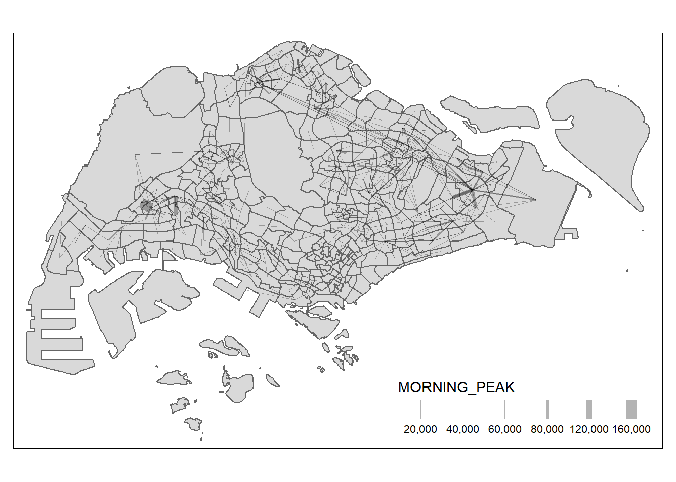
To visualise the resulting desire lines, the code chunk below is used.
tm_shape(mpsz) +
tm_polygons() +
flowLine %>%
tm_shape() +
tm_lines(lwd = "MORNING_PEAK",
style = "quantile",
scale = c(0.1, 1, 3, 5, 7, 10),
n = 6,
alpha = 0.3)
Warning
Be patient, the rendering process takes more time because of the transparency argument (i.e. alpha)
When the flow data are very messy and highly skewed like the one shown above, it is wiser to focus on selected flows, for example flow greater than or equal to 5000 as shown below.
tm_shape(mpsz) +
tm_polygons() +
flowLine %>%
filter(MORNING_PEAK >= 5000) %>%
tm_shape() +
tm_lines(lwd = "MORNING_PEAK",
style = "quantile",
scale = c(0.1, 1, 3, 5, 7, 10),
n = 6,
alpha = 0.3)