pacman::p_load(sf, spatstat, sparr,
tmap, stpp, tidyverse)6 Spatio-Temporal Point Patterns Analysis
6.1 Overview
A spatio-temporal point process (also called space-time or spatial-temporal point process) is a random collection of points, where each point represents the time and location of an event. Examples of events include incidence of disease, sightings or births of a species, or the occurrences of fires, earthquakes, lightning strikes, tsunamis, or volcanic eruptions.
The analysis of spatio-temporal point patterns is becoming increasingly necessary, given the rapid emergence of geographically and temporally indexed data in a wide range of fields. Several spatio-temporal point patterns analysis methods have been introduced and implemented in R in the last ten years. This chapter shows how various R packages can be combined to run a set of spatio-temporal point pattern analyses in a guided and intuitive way. A real world forest fire events in Kepulauan Bangka Belitung, Indonesia from 1st January 2023 to 31st December 2023 is used to illustrate the methods, procedures and interpretations.
6.2 Learning Outcome
6.2.1 The research questions
The specific questions we would like to answer are:
- are the locations of forest fire in Kepulauan Bangka Belitung spatial and spatio-temporally independent?
- if the answer is NO, where and when the observed forest fire locations tend to cluster?
6.3 The data
For the purpose of this exercise, two data sets will be used, they are:
- forestfires, a csv file provides locations of forest fire detected from the Moderate Resolution Imaging Spectroradiometer (MODIS) sensor data. The data are downloaded from Fire Information for Resource Management System. For the purpose of this exercise, only forest fires within Kepulauan Bangka Belitung will be used.
- Kepulauan_Bangka_Belitung, an ESRI shapefile showing the sub-district (i.e. kelurahan) boundary of Kepulauan Bangka Belitung. The data set was downloaded from Indonesia Geospatial portal. The original data covers the whole Indonesia. For the purpose of this exercise, only sub-districts within Kepulauan Bangka Belitung are extracted.
6.4 Installing and Loading the R packages
For the purpose of this study, six R packages will be used. They are:
- sf provides functions for importing processing and wrangling geospatial data,,
- raster for handling raster data in R,
- spatstat for performing Spatial Point Patterns Analysis such as kcross, Lcross, etc.,
- sparr provides functions to estimate fixed and adaptive kernel-smoothed spatial relative risk surfaces via the density-ratio method and perform subsequent inference. Fixed-bandwidth spatiotemporal density and relative risk estimation is also supported
- tmap provides functions to produce cartographic quality thematic maps, and
- tidyverse, a family of R packages that provide functions to perform common data science tasks including and not limited to data import, data transformation, data wrangling and data visualisation.
Using the steps you learned from previous chapter, write a code chunk to load the packages above onto R environment.
6.5 Importing and Preparing Study Area
6.5.1 Importing study area
Code chunk below is used import study area (i.e. Kepulauan Bangka Belitung) into R environment.
kbb <- st_read(dsn="chap06/data/rawdata",
               layer = "Kepulauan_Bangka_Belitung")
The revised code chunk.
kbb_sf <- st_read(dsn="chap06/data/rawdata",
               layer = "Kepulauan_Bangka_Belitung") %>%
  st_union() %>%
  st_zm(drop = TRUE, what = "ZM") %>%
  st_transform(crs = 32748)
Reading layer `Kepulauan_Bangka_Belitung' from data source
`C:\tskam\r4gdsa\chap06\data\rawdata' using driver `ESRI Shapefile'
Simple feature collection with 297 features and 26 fields
Geometry type: POLYGON
Dimension: XYZ
Bounding box: xmin: 105.1085 ymin: -3.116593 xmax: 106.8488 ymax: -1.501603
z_range: zmin: 0 zmax: 0
Geodetic CRS: WGS 846.5.2 Converting OWIN
Next, as.owin() is used to convert kbb into an owin object.
kbb_owin <- as.owin(kbb_sf)
kbb_owin
window: polygonal boundary
enclosing rectangle: [512066.8, 705559.4] x [9655398, 9834006] unitsNext, class() is used to confirm if the output is indeed an owin object.
class(kbb_owin)[1] "owin"6.6 Importing and Preparing Forest Fire data
Next, we will import the forest fire data set (i.e. forestfires.csv) into R environment.
fire_sf <- read_csv("chap06/data/rawdata/forestfires.csv") %>%
  st_as_sf(coords = c("longitude", "latitude"),
                       crs = 4326) %>%
  st_transform(crs = 32748)
Because ppp object only accept numerical or character as mark. The code chunk below is used to convert data type of acq_date to numeric.
fire_sf <- fire_sf %>%
  mutate(DayofYear = yday(acq_date)) %>%
  mutate(Month_num = month(acq_date)) %>%
  mutate(Month_fac = month(acq_date,
                           label = TRUE,
                           abbr = FALSE))
6.7 Visualising the Fire Points
6.7.1 Overall plot
Using the steps you learned in Hands-on Exercise 2, prepare a point symbol map showing the distribution of fire points. The map should look similar to the figure below.
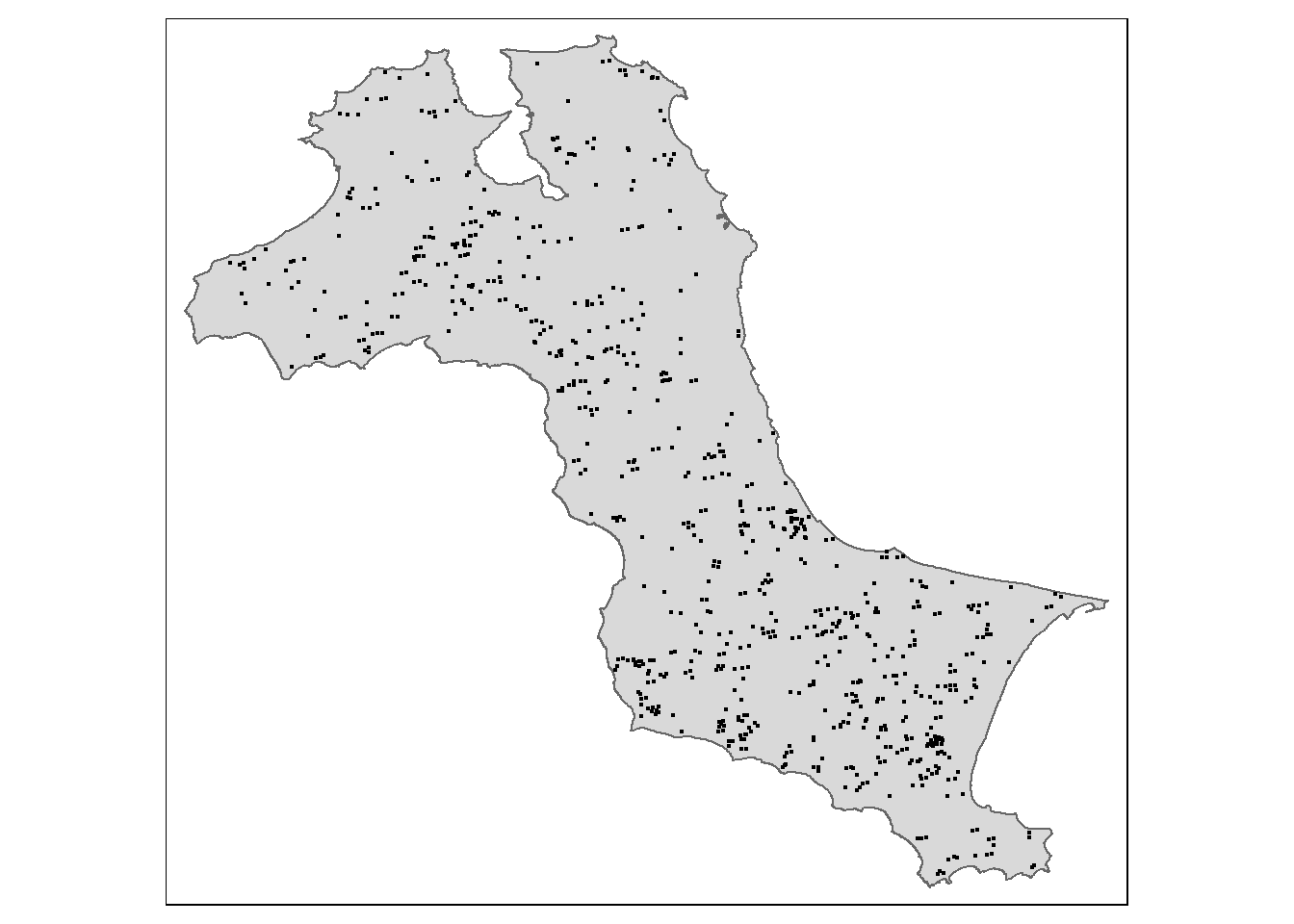
tm_shape(kbb_sf)+
  tm_polygons() +
tm_shape(fire_sf) +
  tm_dots()
6.7.2 Visuaising geographic distribution of forest fires by month
Using the steps you learned in Hands-on Exercise 2, prepare a point symbol map showing the monthly geographic distribution of forest fires in 2023. The map should look similar to the figure below.
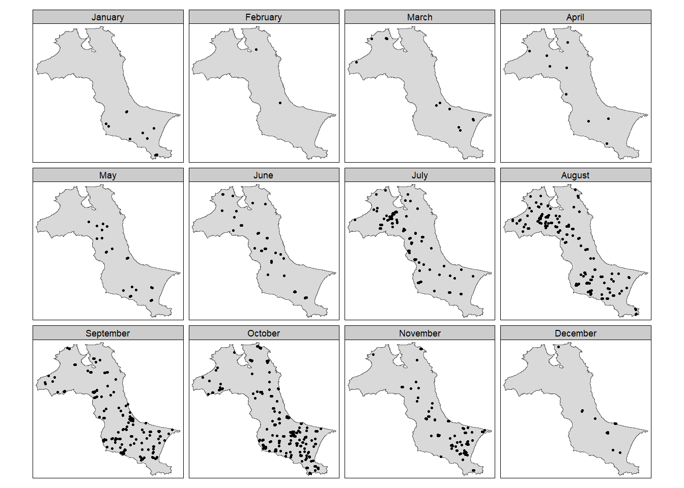
tm_shape(kbb_sf)+
  tm_polygons() +
tm_shape(fire_sf) +
  tm_dots(size = 0.1) +
tm_facets(by="Month_fac",
            free.coords=FALSE,
            drop.units = TRUE)
6.8 Computing STKDE by Month
In this section, you will learn how to compute STKDE by using spattemp.density() of sparr package. Before using the function, it is highly recommended you read the function’s reference guide in detail in order to understand the input data requirements and the output object generated.
6.8.1 Extracting forest fires by month
The code chunk below is used to remove the unwanted fields from fire_sf sf data.frame. This is because as.ppp() only need the mark field and geometry field from the input sf data.frame.
fire_month <- fire_sf %>%
  select(Month_num)
6.8.2 Creating ppp
The code chunk below is used to derive a ppp object called fire_month from fire_month sf data.frame.
fire_month_ppp <- as.ppp(fire_month)
fire_month_ppp
Marked planar point pattern: 741 points
marks are numeric, of storage type 'double'
window: rectangle = [521564.1, 695791] x [9658137, 9828767] unitsThe code chunk below is used to check the output is in the correct object class.
summary(fire_month_ppp)Marked planar point pattern: 741 points
Average intensity 2.49258e-08 points per square unit
Coordinates are given to 10 decimal places
marks are numeric, of type 'double'
Summary:
Min. 1st Qu. Median Mean 3rd Qu. Max.
1.000 8.000 9.000 8.579 10.000 12.000
Window: rectangle = [521564.1, 695791] x [9658137, 9828767] units
(174200 x 170600 units)
Window area = 29728200000 square unitsNext, we will check if there are duplicated point events by using the code chunk below.
any(duplicated(fire_month_ppp))[1] FALSE6.8.3 Including Owin object
The code chunk below is used to combine origin_am_ppp and am_owin objects into one.
fire_month_owin <- fire_month_ppp[kbb_owin]
summary(fire_month_owin)
Marked planar point pattern: 741 points
Average intensity 6.42469e-08 points per square unit
Coordinates are given to 10 decimal places
marks are numeric, of type 'double'
Summary:
Min. 1st Qu. Median Mean 3rd Qu. Max.
1.000 8.000 9.000 8.579 10.000 12.000
Window: polygonal boundary
single connected closed polygon with 47493 vertices
enclosing rectangle: [512066.8, 705559.4] x [9655398, 9834006] units
(193500 x 178600 units)
Window area = 11533600000 square units
Fraction of frame area: 0.334As a good practice, plot() is used to plot ff_owin so that we can examine the correctness of the output object.
plot(fire_month_owin)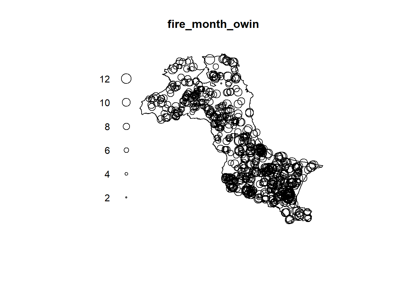
6.8.4 Computing Spatio-temporal KDE
Next, spattemp.density() of sparr package is used to compute the STKDE.
st_kde <- spattemp.density(fire_month_owin)
summary(st_kde)
Spatiotemporal Kernel Density Estimate
Bandwidths
h = 15102.47 (spatial)
lambda = 0.0304 (temporal)
No. of observations
741
Spatial bound
Type: polygonal
2D enclosure: [512066.8, 705559.4] x [9655398, 9834006]
Temporal bound
[1, 12]
Evaluation
128 x 128 x 12 trivariate lattice
Density range: [1.233458e-27, 8.202976e-10]6.8.5 Plotting the spatio-temporal KDE object
In the code chunk below, plot() of R base is used to the KDE for between July 2023 - December 2023.
tims <- c(7,8,9,10,11,12)
par(mfcol=c(2,3))
for(i in tims){
  plot(st_kde, i,
       override.par=FALSE,
       fix.range=TRUE,
       main=paste("KDE at month",i))
}
6.9 Computing STKDE by Day of Year
In this section, you will learn how to computer the STKDE of forest fires by day of year.
6.9.1 Creating ppp object
In the code chunk below, DayofYear field is included in the output ppp object.
fire_yday_ppp <- fire_sf %>%
  select(DayofYear) %>%
  as.ppp()
6.9.2 Including Owin object
Next, code chunk below is used to combine the ppp object and the owin object.
fire_yday_owin <- fire_yday_ppp[kbb_owin]
summary(fire_yday_owin)
Marked planar point pattern: 741 points
Average intensity 6.42469e-08 points per square unit
Coordinates are given to 10 decimal places
marks are numeric, of type 'double'
Summary:
Min. 1st Qu. Median Mean 3rd Qu. Max.
10.0 213.0 258.0 245.9 287.0 352.0
Window: polygonal boundary
single connected closed polygon with 47493 vertices
enclosing rectangle: [512066.8, 705559.4] x [9655398, 9834006] units
(193500 x 178600 units)
Window area = 11533600000 square units
Fraction of frame area: 0.3346.9.3
kde_yday <- spattemp.density(
  fire_yday_owin)
summary(kde_yday)
Spatiotemporal Kernel Density Estimate
Bandwidths
h = 15102.47 (spatial)
lambda = 6.3198 (temporal)
No. of observations
741
Spatial bound
Type: polygonal
2D enclosure: [512066.8, 705559.4] x [9655398, 9834006]
Temporal bound
[10, 352]
Evaluation
128 x 128 x 343 trivariate lattice
Density range: [3.959516e-27, 2.751287e-12]plot(kde_yday)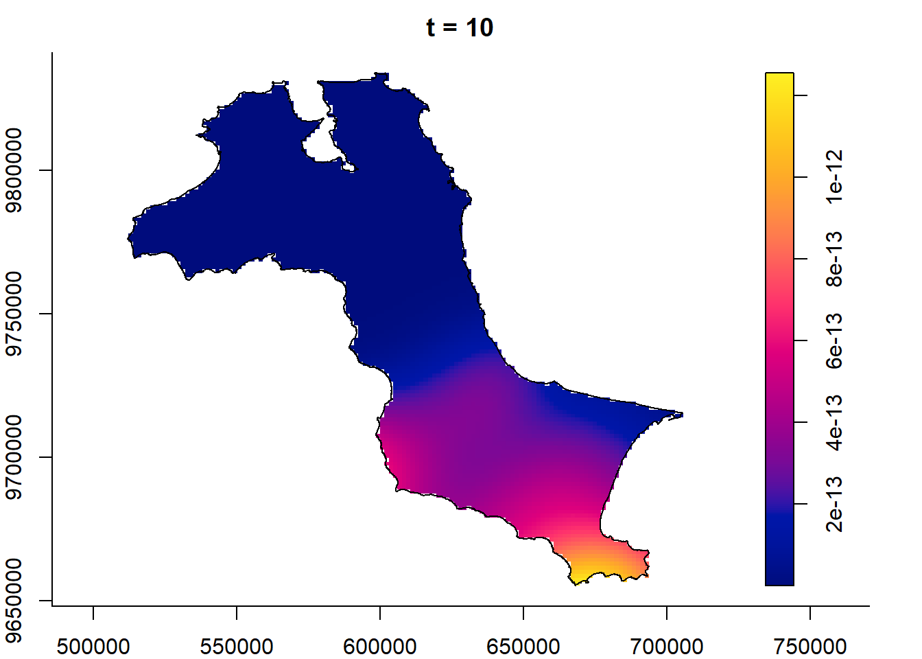


6.10 Computing STKDE by Day of Year: Improved method
One of the nice function provides in sparr package is BOOT.spattemp(). It support bandwidth selection for standalone spatiotemporal density/intensity based on bootstrap estimation of the MISE, providing an isotropic scalar spatial bandwidth and a scalar temporal bandwidth.
Code chunk below uses BOOT.spattemp() to determine both the spatial bandwidth and the scalar temporal bandwidth.
set.seed(1234)
BOOT.spattemp(fire_yday_owin)
Initialising...Done.
Optimising...
h = 15102.47 ; lambda = 16.84806
h = 16612.72 ; lambda = 16.84806
h = 15102.47 ; lambda = 1527.095
h = 15480.03 ; lambda = 771.9715
h = 15668.81 ; lambda = 394.4098
h = 15763.2 ; lambda = 205.6289
h = 15810.4 ; lambda = 111.2385
h = 15833.99 ; lambda = 64.04328
h = 15845.79 ; lambda = 40.44567
h = 15851.69 ; lambda = 28.64687
h = 15863.49 ; lambda = 5.049258
h = 15854.64 ; lambda = 22.74746
h = 15860.54 ; lambda = 10.94866
h = 15859.07 ; lambda = 13.89836
h = 14348.82 ; lambda = 13.89836
h = 13216.87 ; lambda = 12.42351
h = 12460.27 ; lambda = 15.37321
h = 10760.88 ; lambda = 16.11064
h = 8875.282 ; lambda = 11.68608
h = 10432.08 ; lambda = 12.97658
h = 7976.084 ; lambda = 16.66371
h = 9286.281 ; lambda = 15.60366
h = 9615.08 ; lambda = 18.73771
h = 9206.581 ; lambda = 21.61828
h = 8140.483 ; lambda = 18.23073
h = 8795.582 ; lambda = 17.70071
h = 9124.381 ; lambda = 20.83477
h = 9164.856 ; lambda = 19.52699
h = 8345.358 ; lambda = 18.48998
h = 9297.65 ; lambda = 18.67578
h = 8928.375 ; lambda = 16.8495
h = 9105.736 ; lambda = 18.85762
Done. h lambda
9105.73611 18.85762 6.10.1 Computing spatio-temporal KDE
Now, the STKDE will be derived by using h and lambda values derive in previous step.
kde_yday <- spattemp.density(fire_yday_owin,
                             h = 9000,
                             lambda = 19)
summary(kde_yday)
Spatiotemporal Kernel Density Estimate
Bandwidths
h = 9000 (spatial)
lambda = 19 (temporal)
No. of observations
741
Spatial bound
Type: polygonal
2D enclosure: [512066.8, 705559.4] x [9655398, 9834006]
Temporal bound
[10, 352]
Evaluation
128 x 128 x 343 trivariate lattice
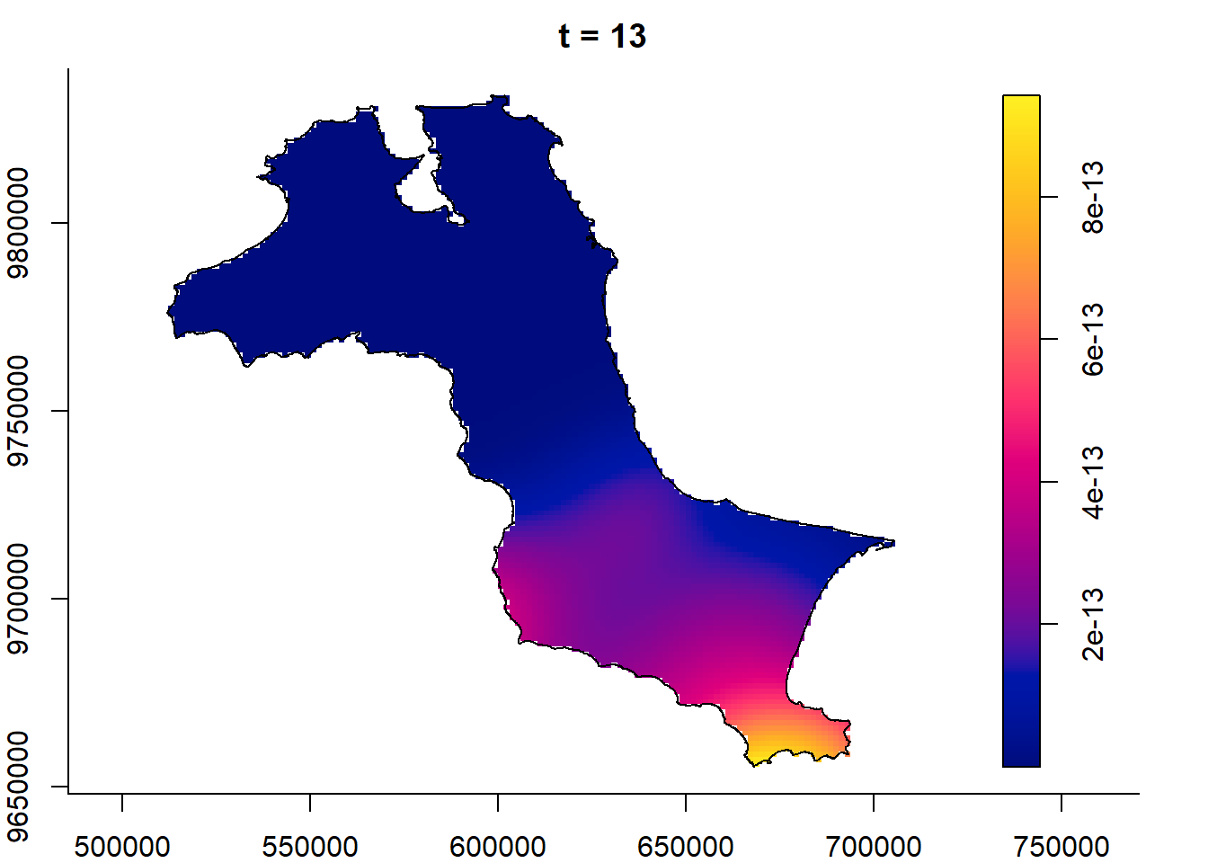
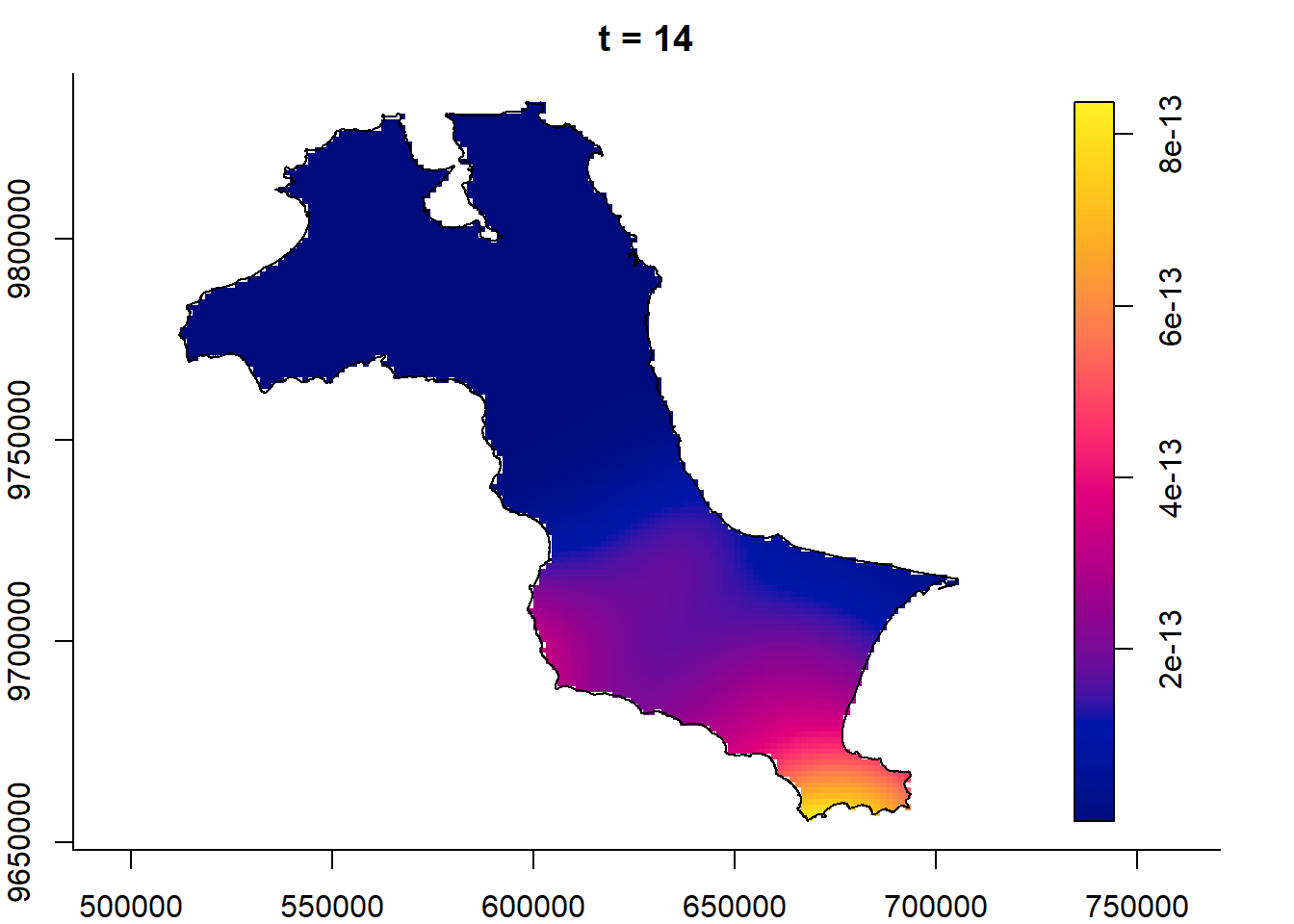
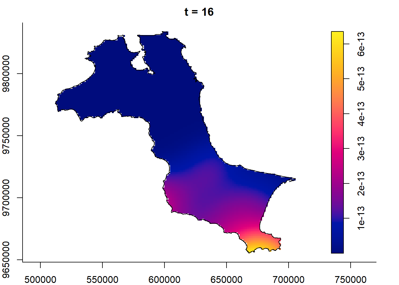
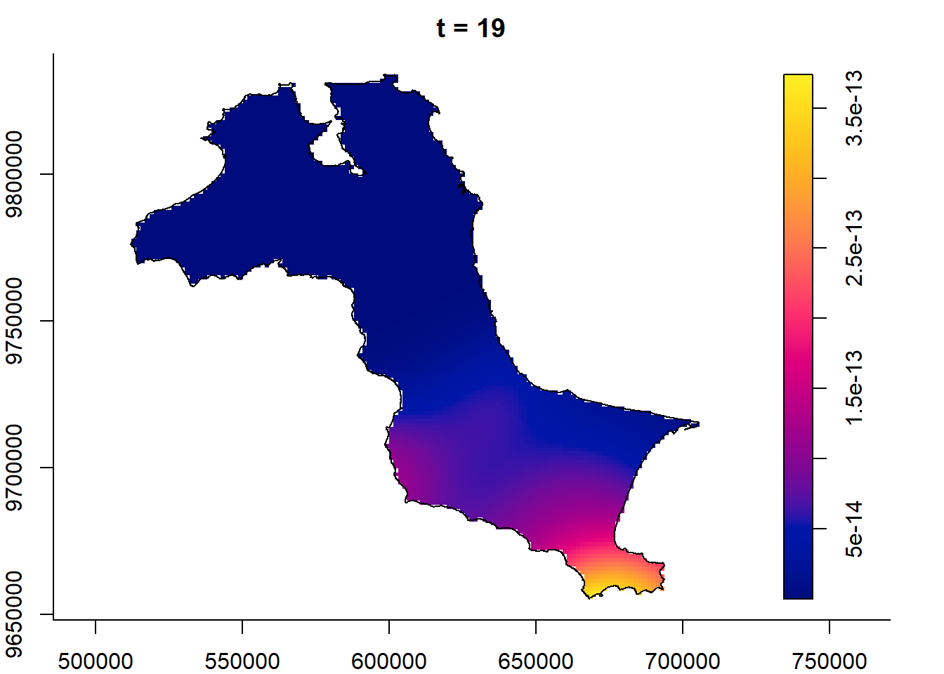
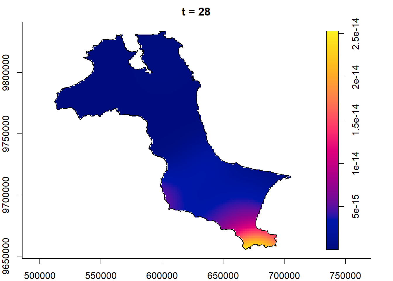
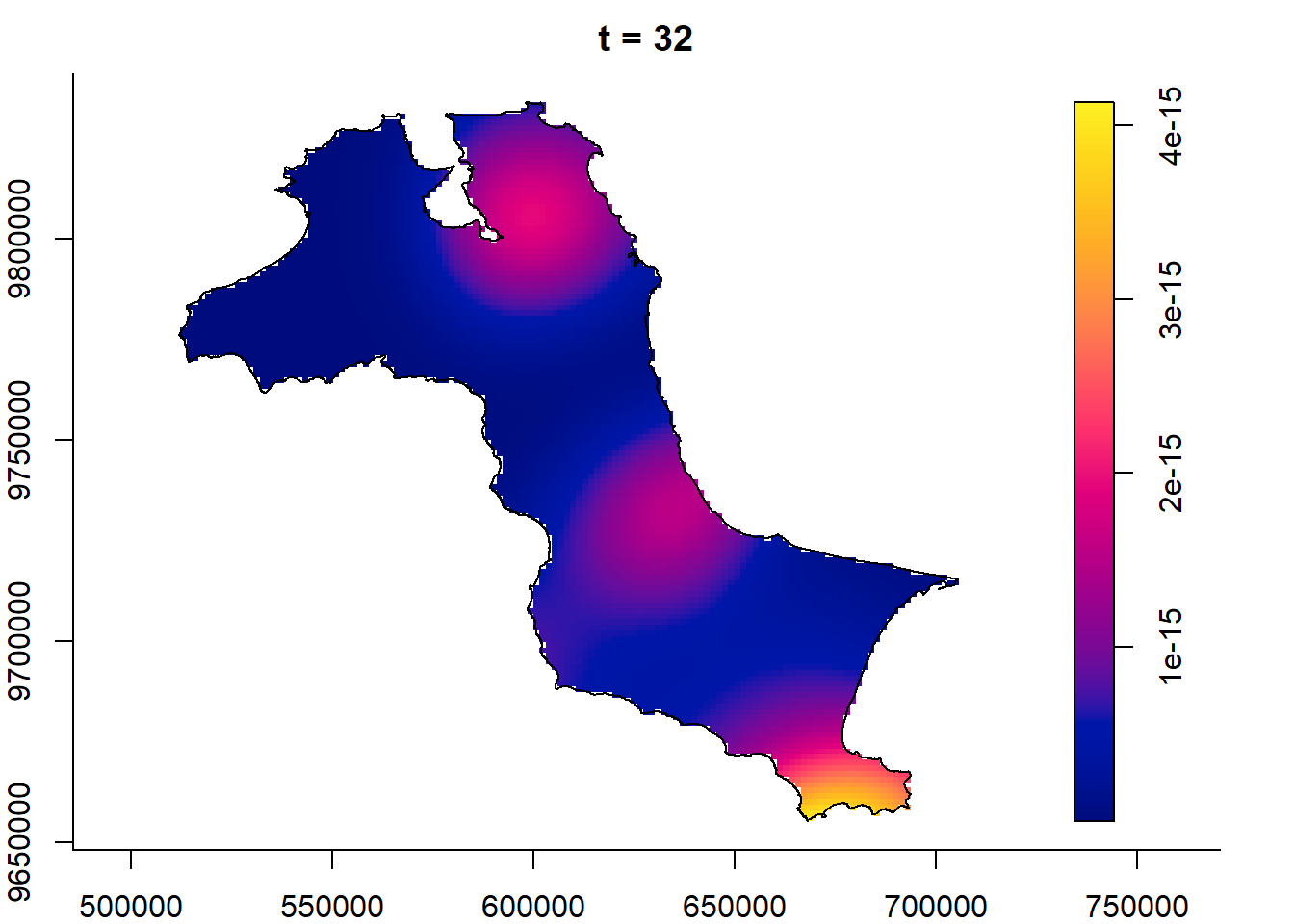
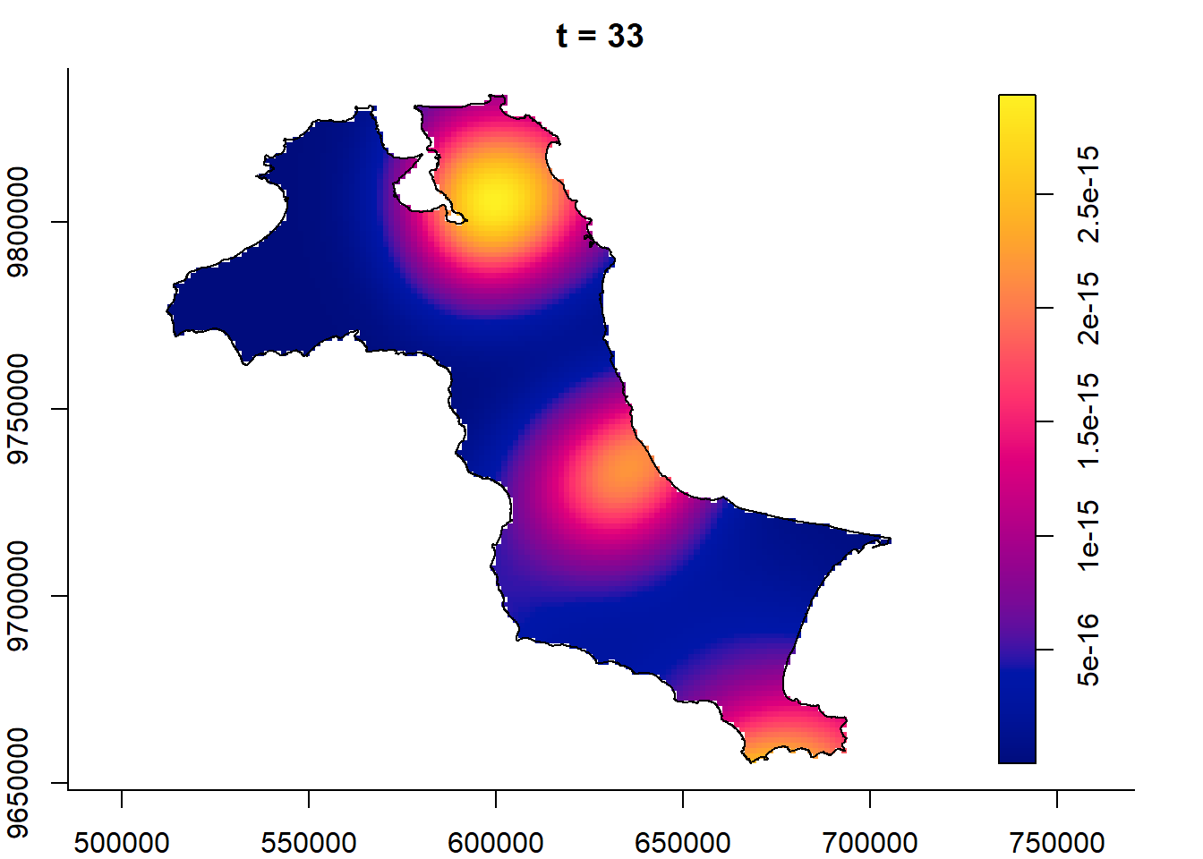
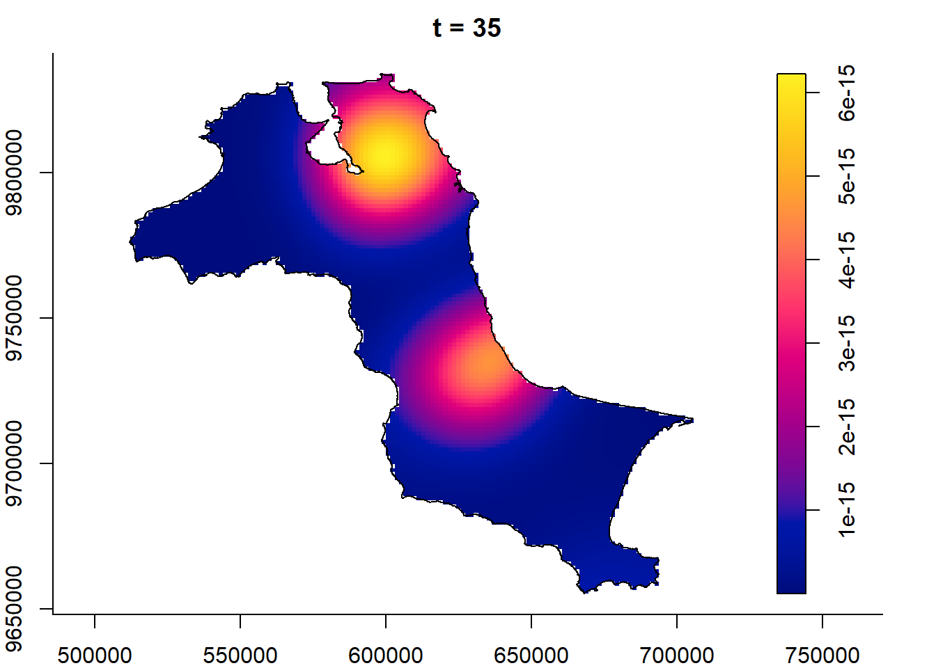
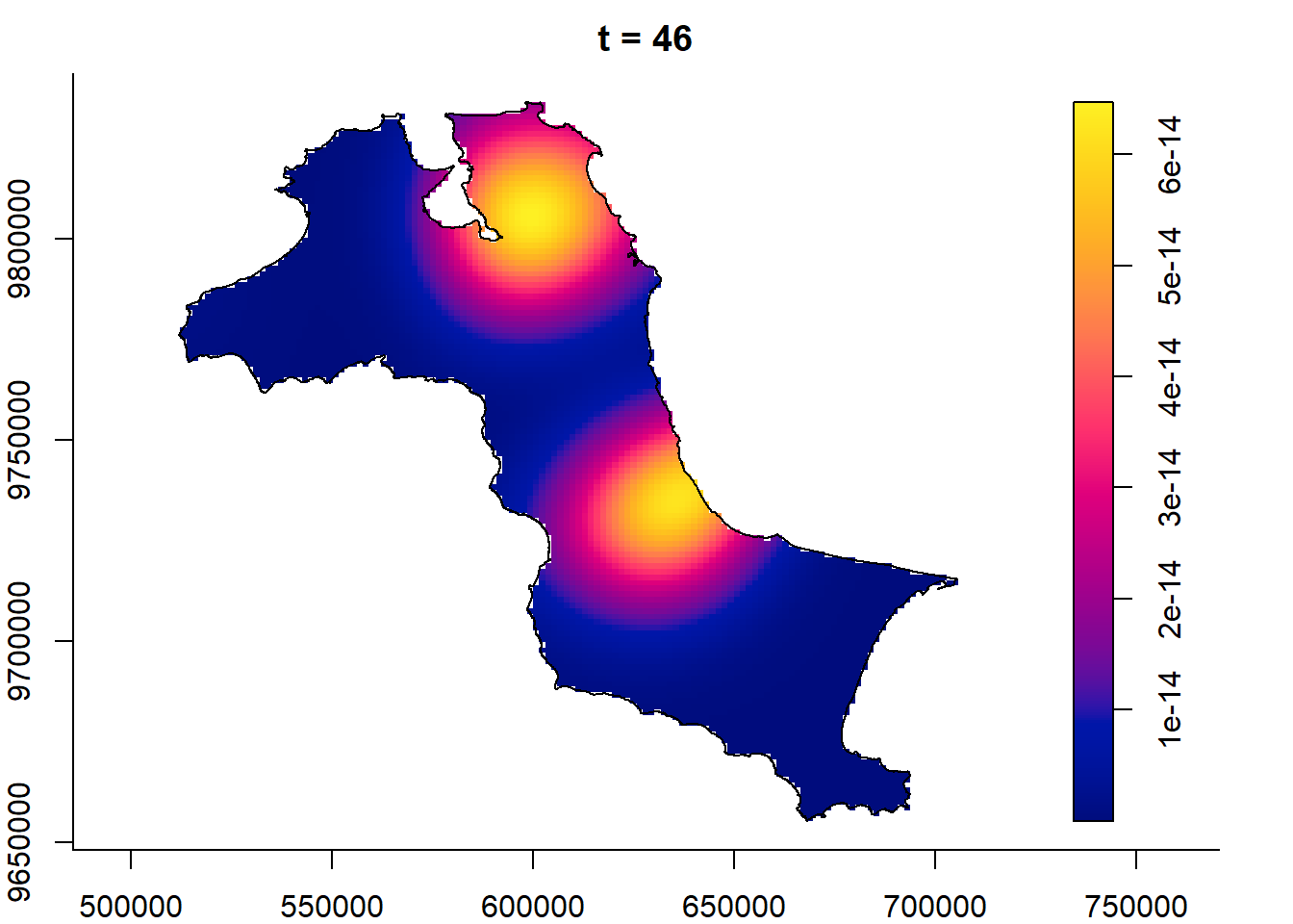
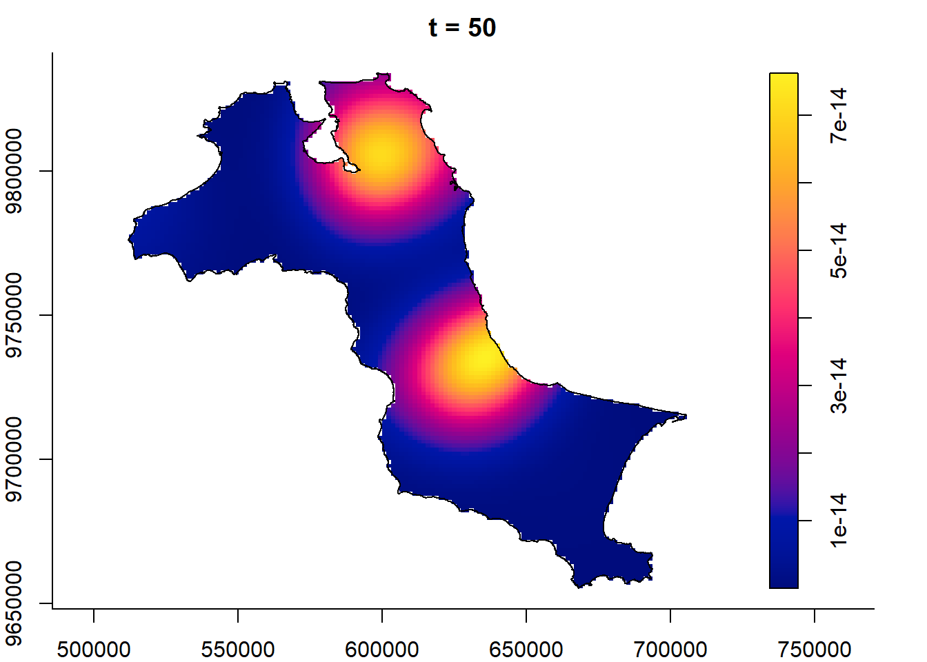
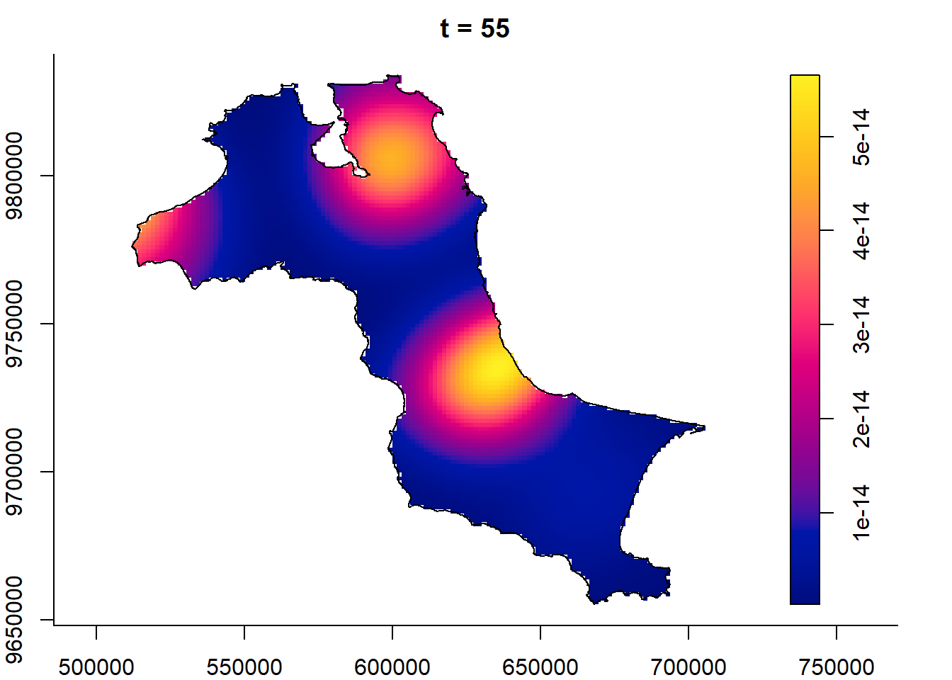
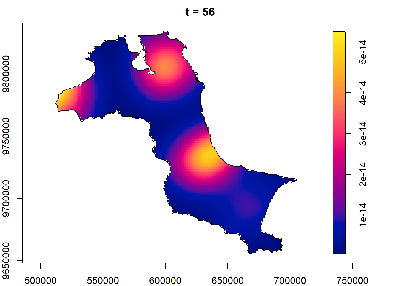
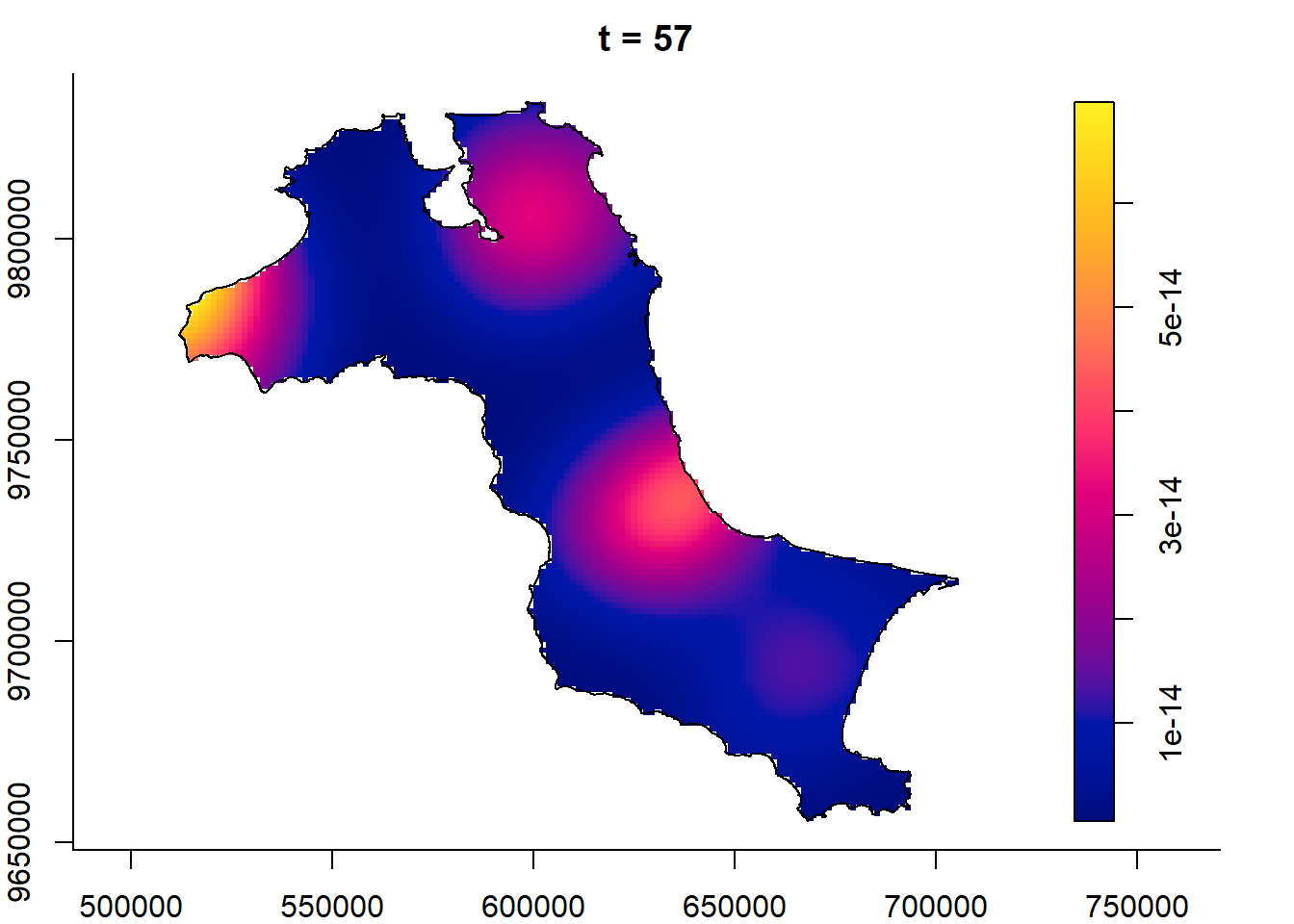
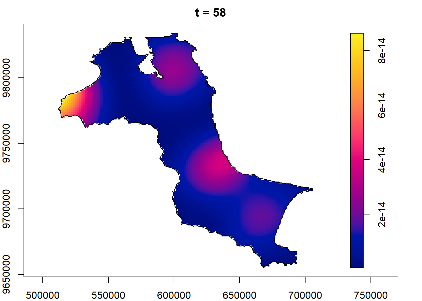
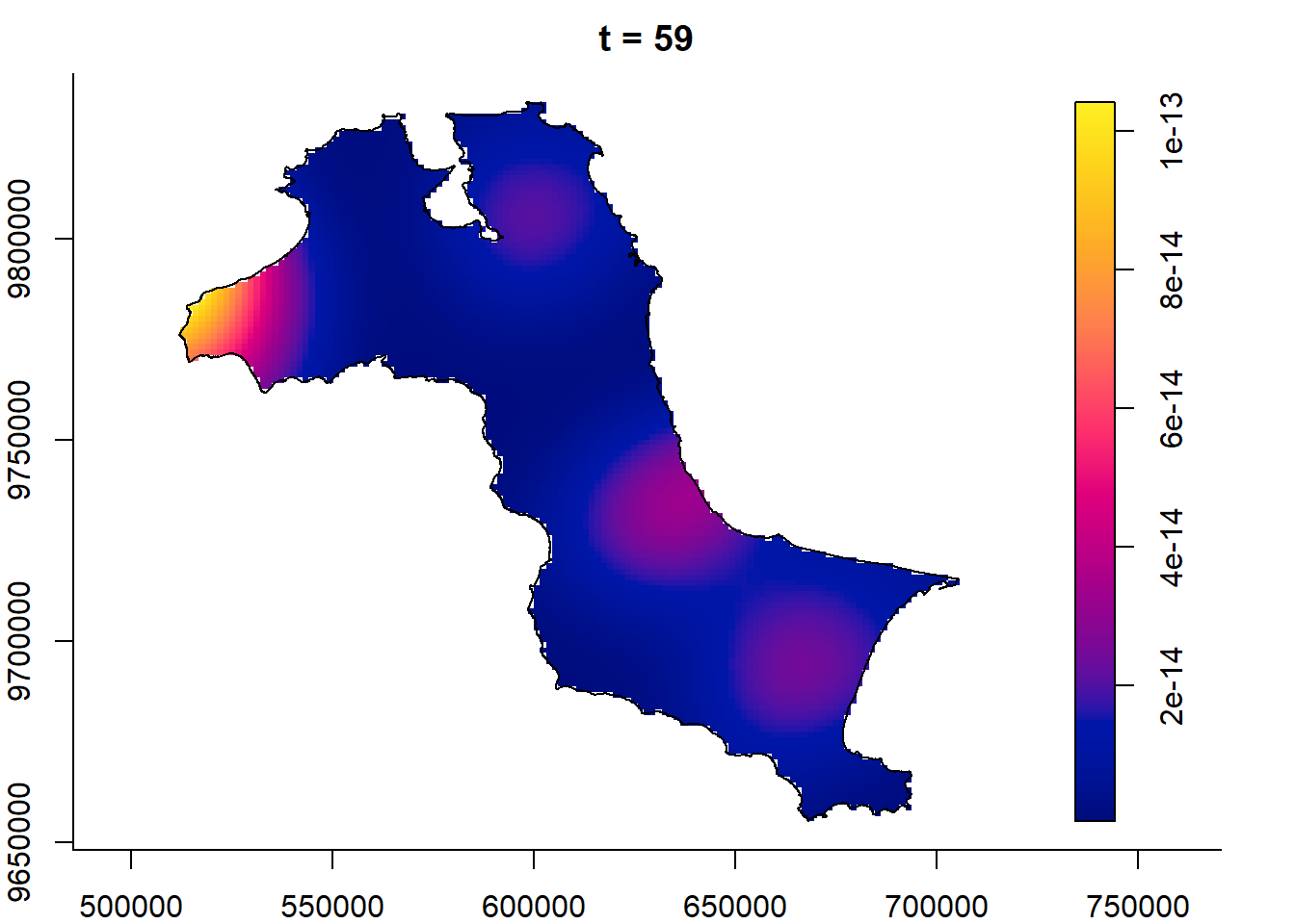
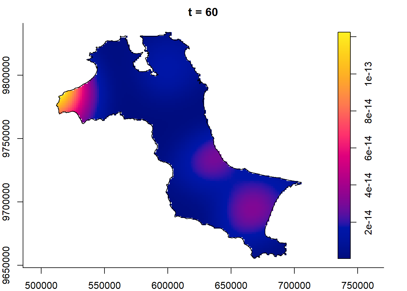
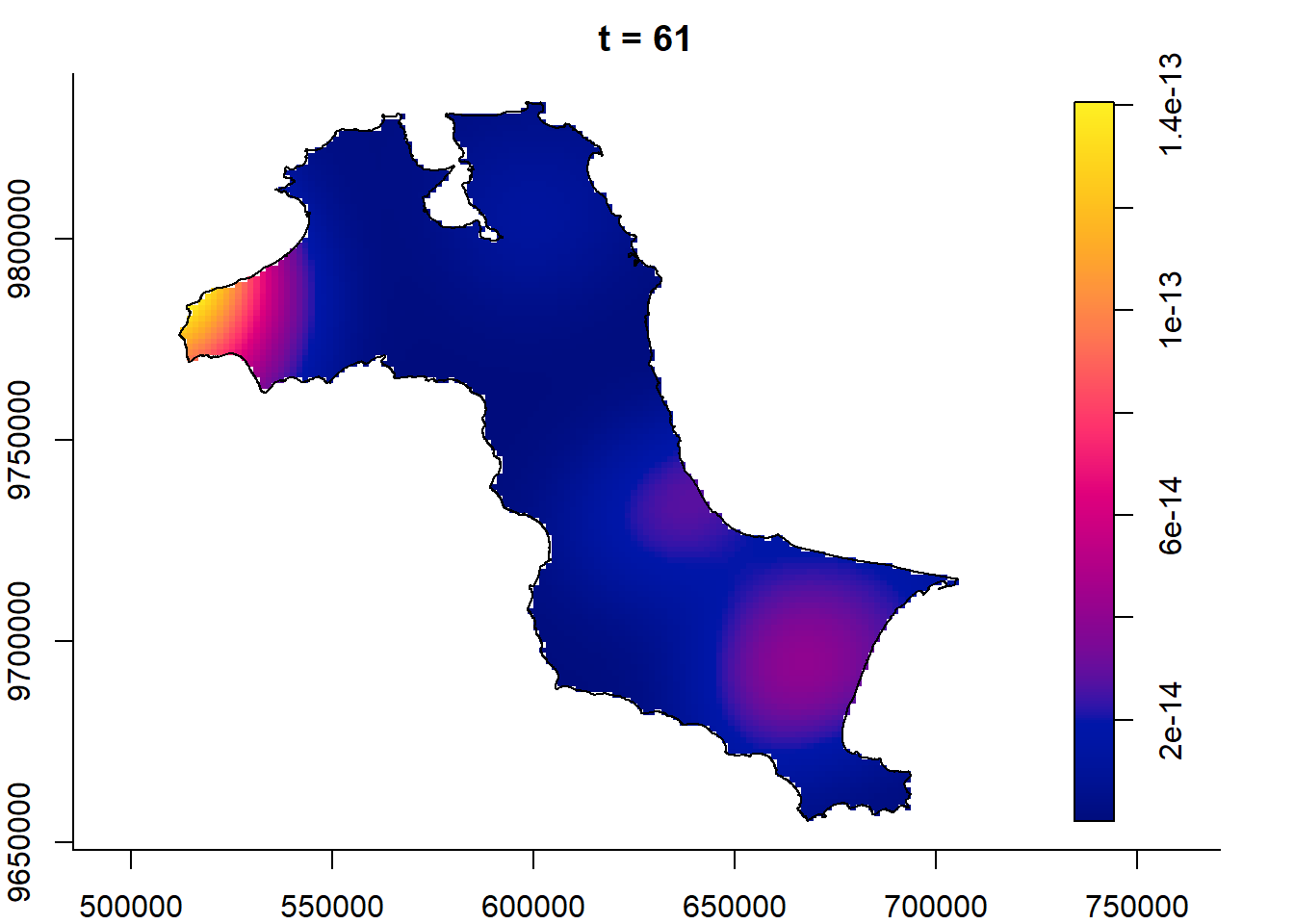
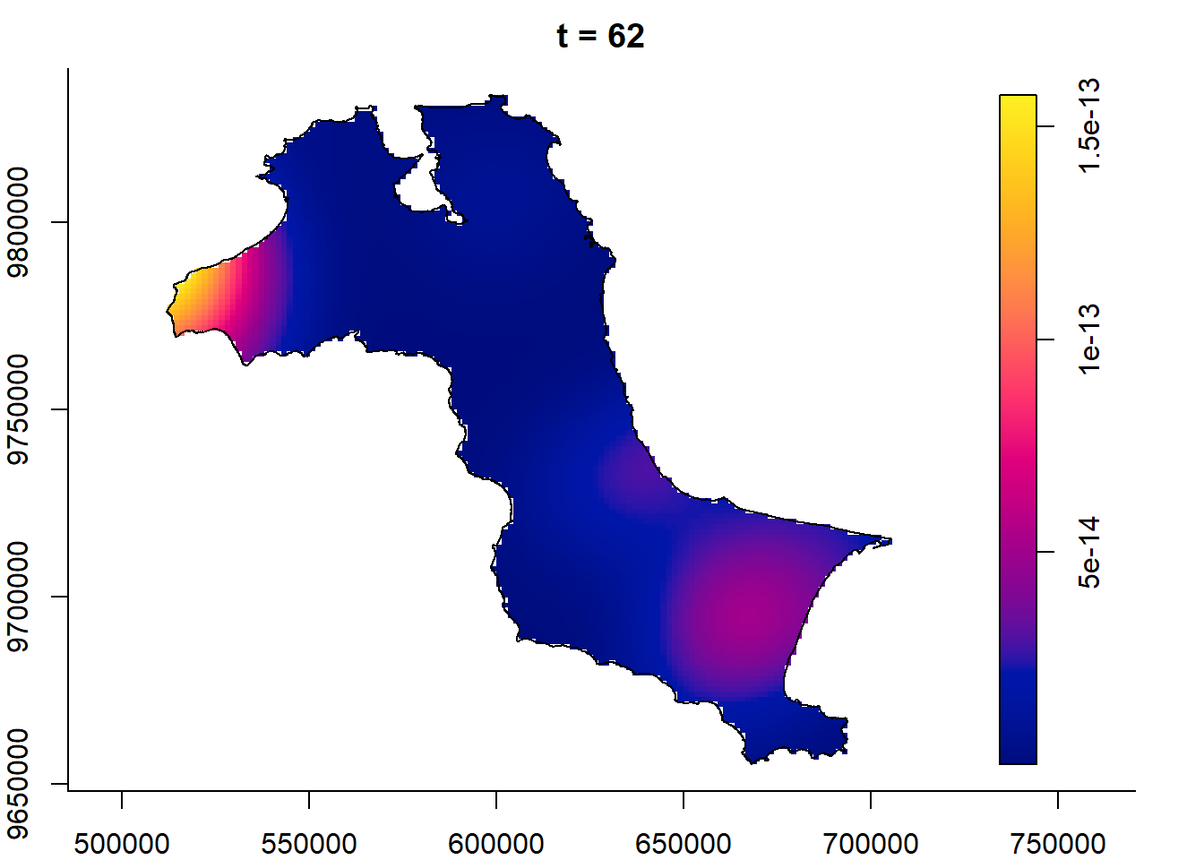
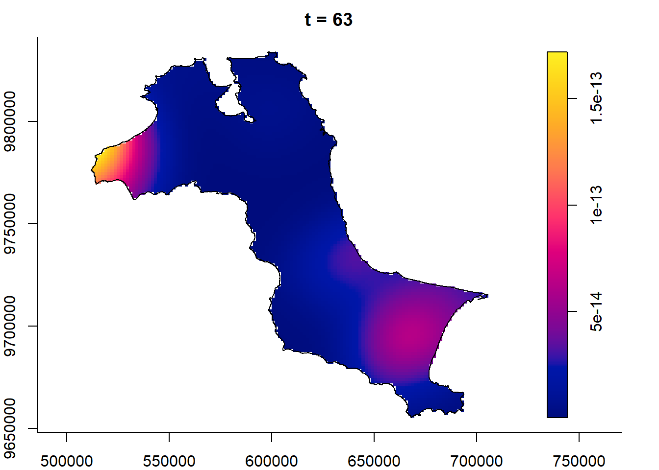
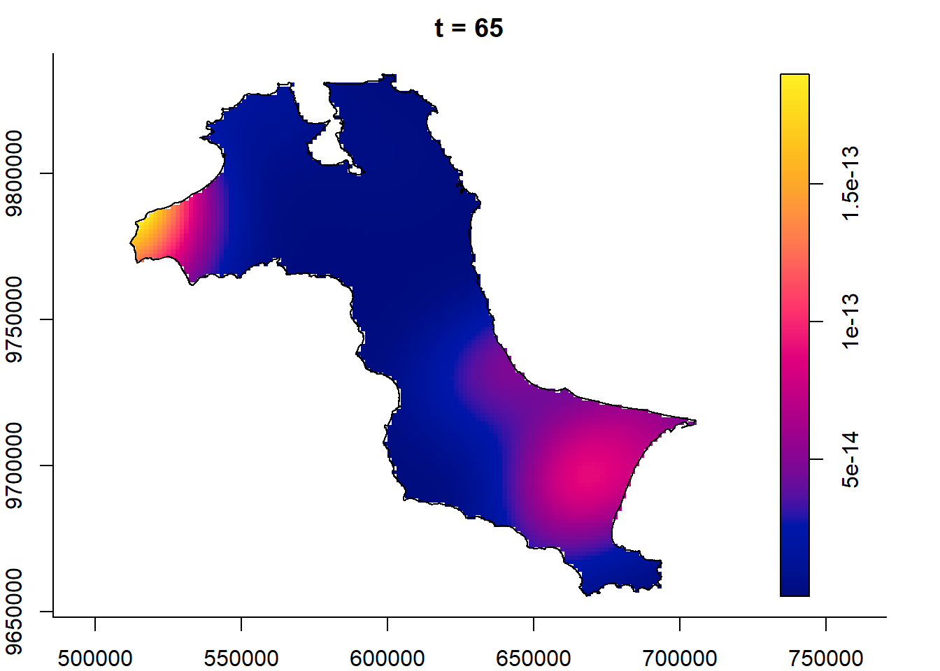
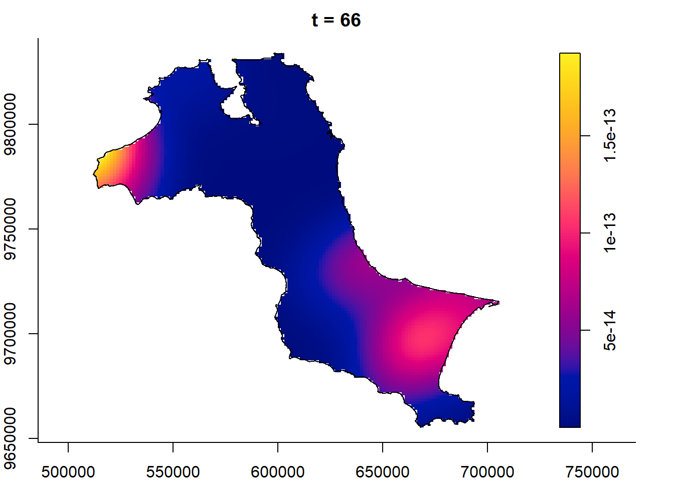
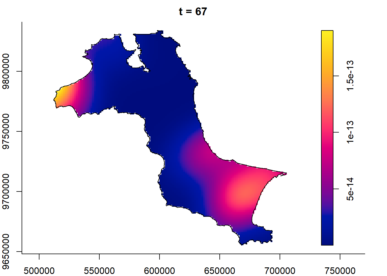
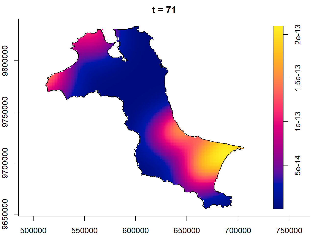
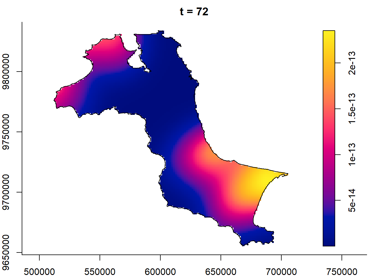
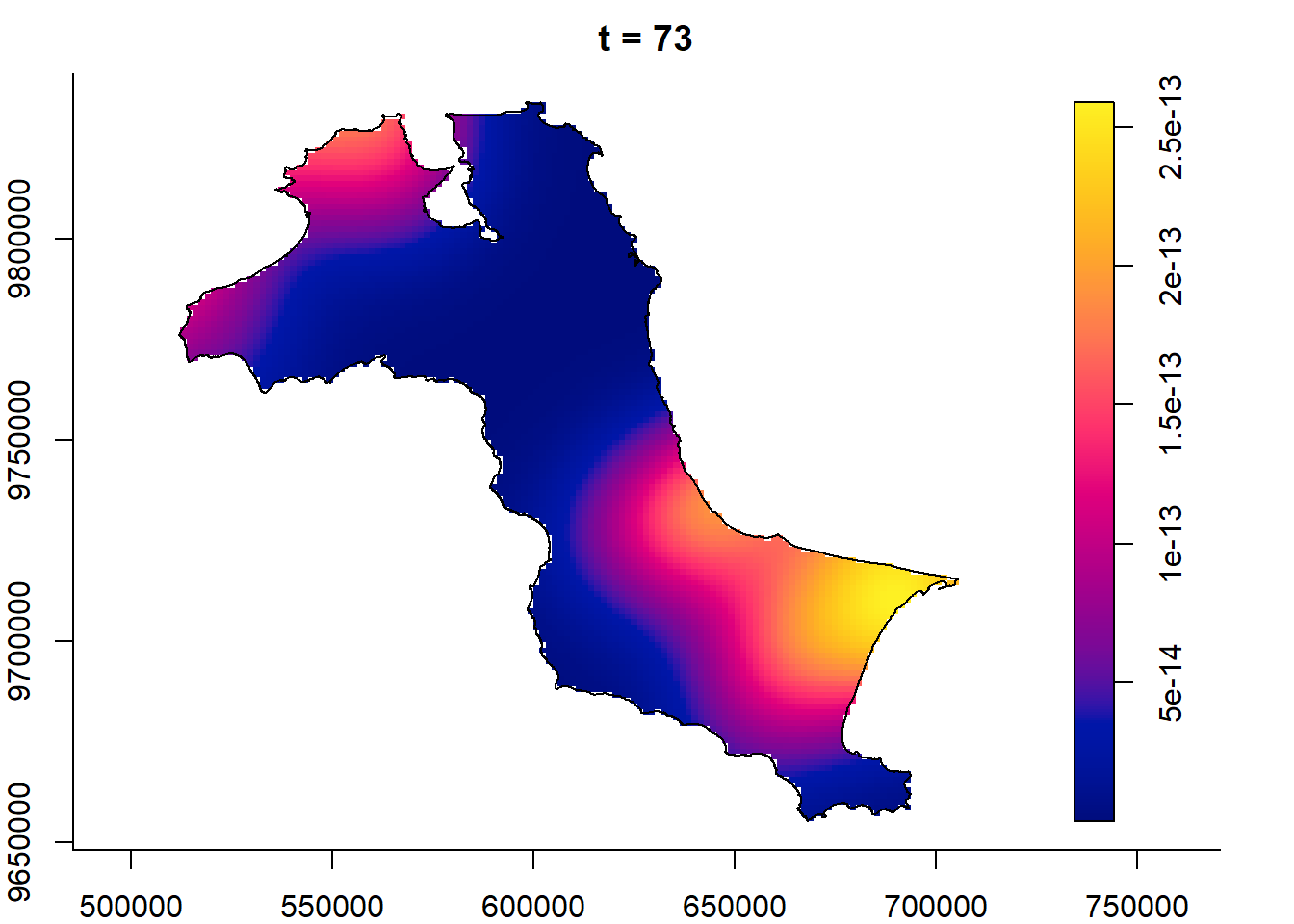
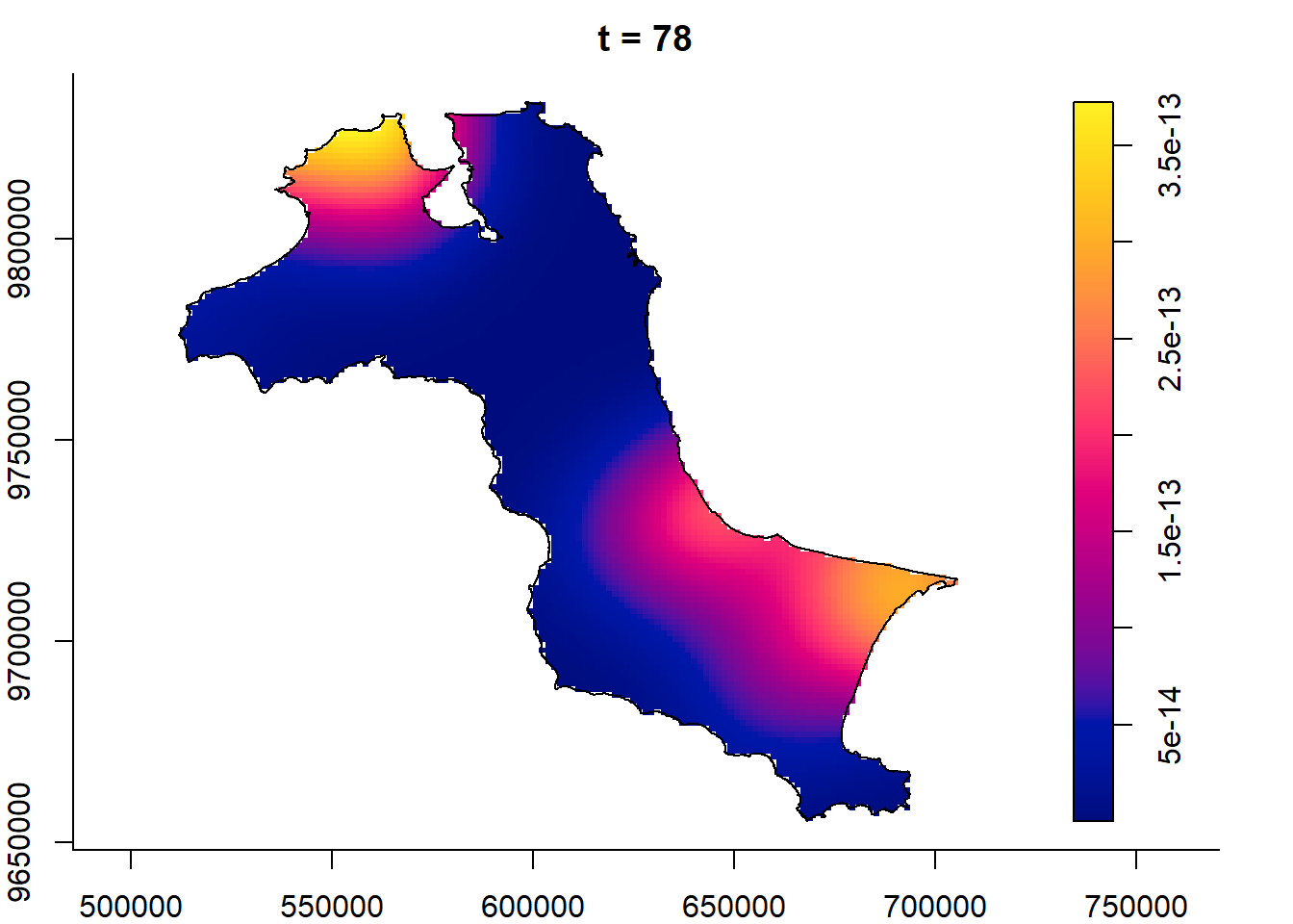
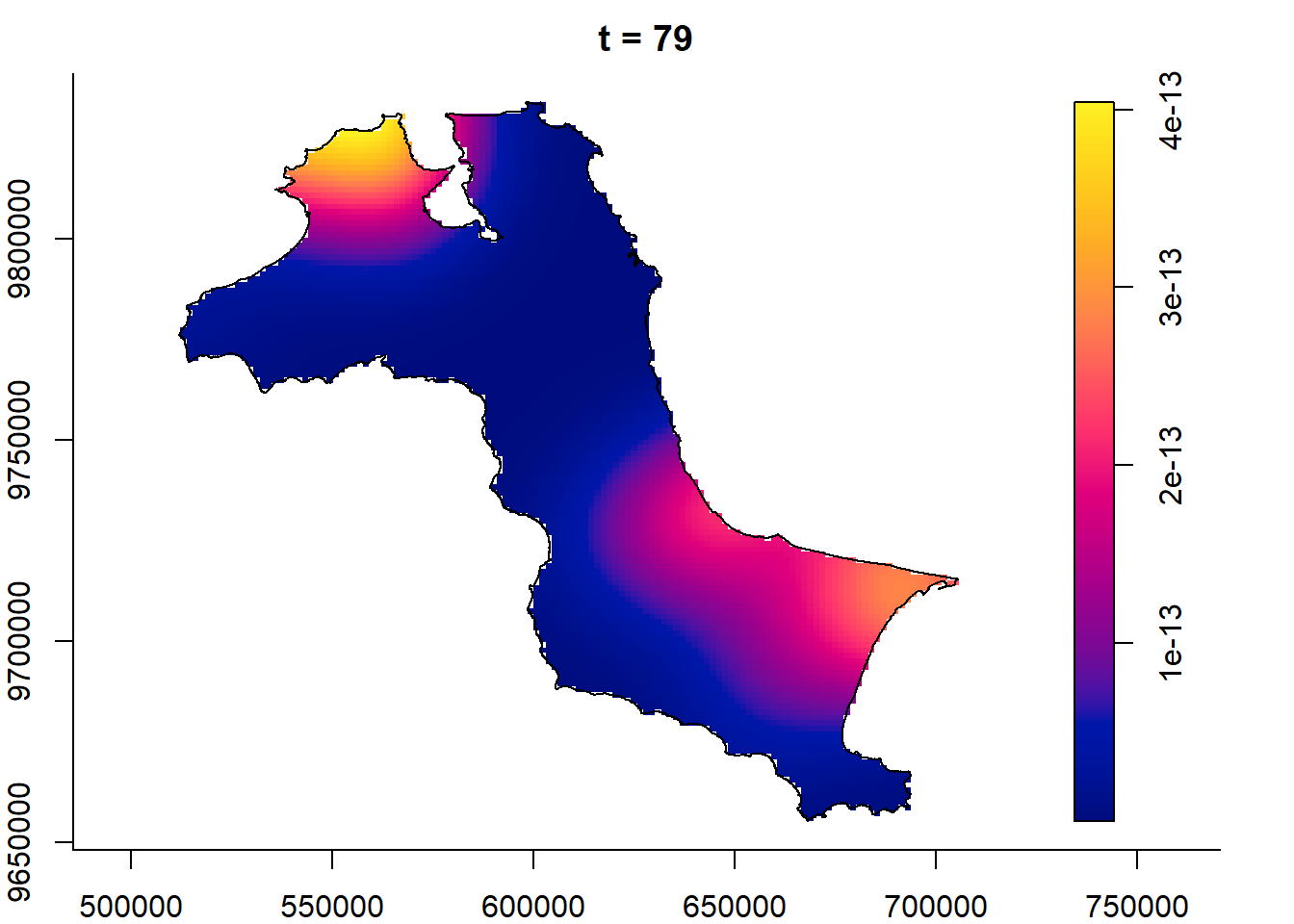
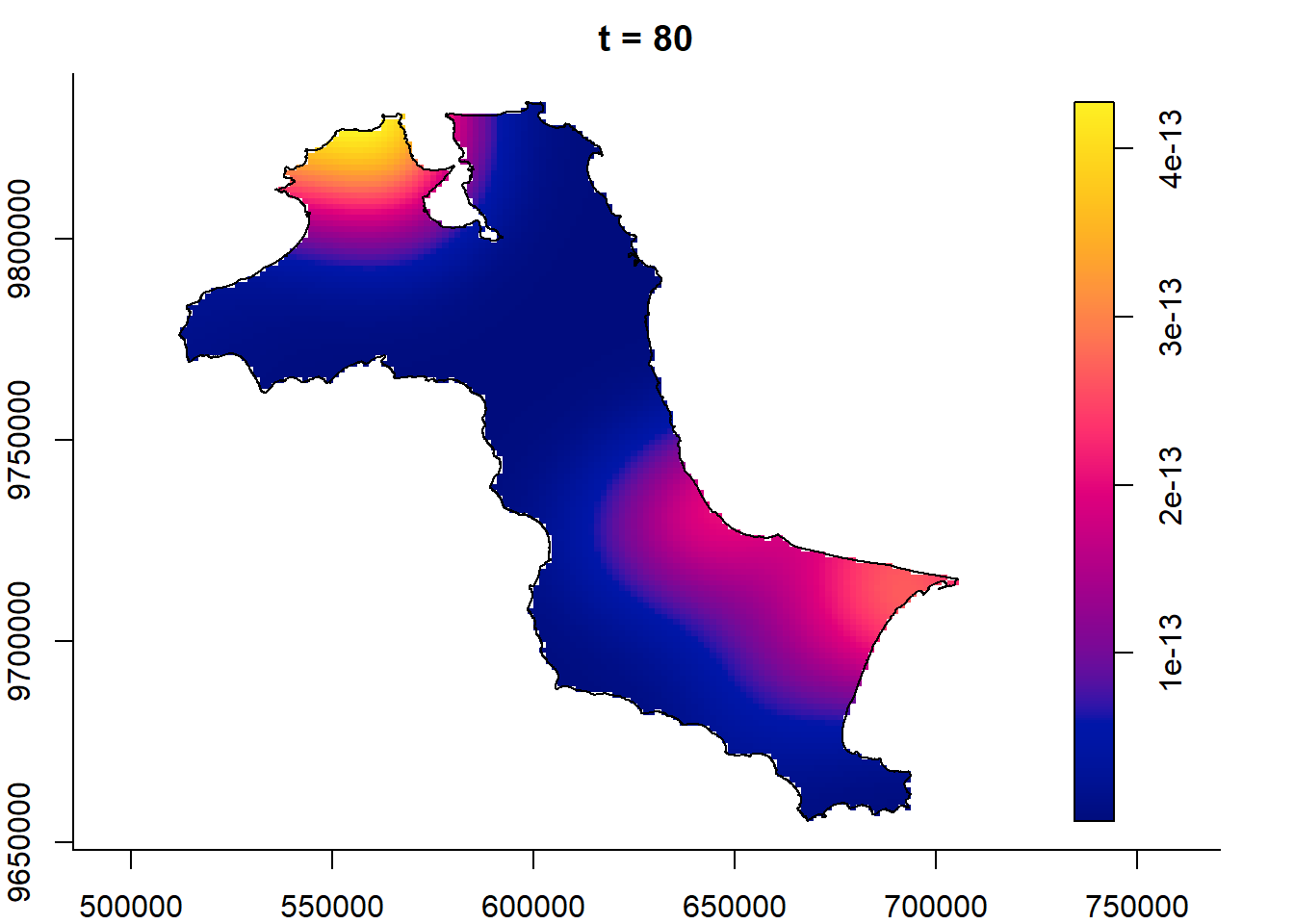
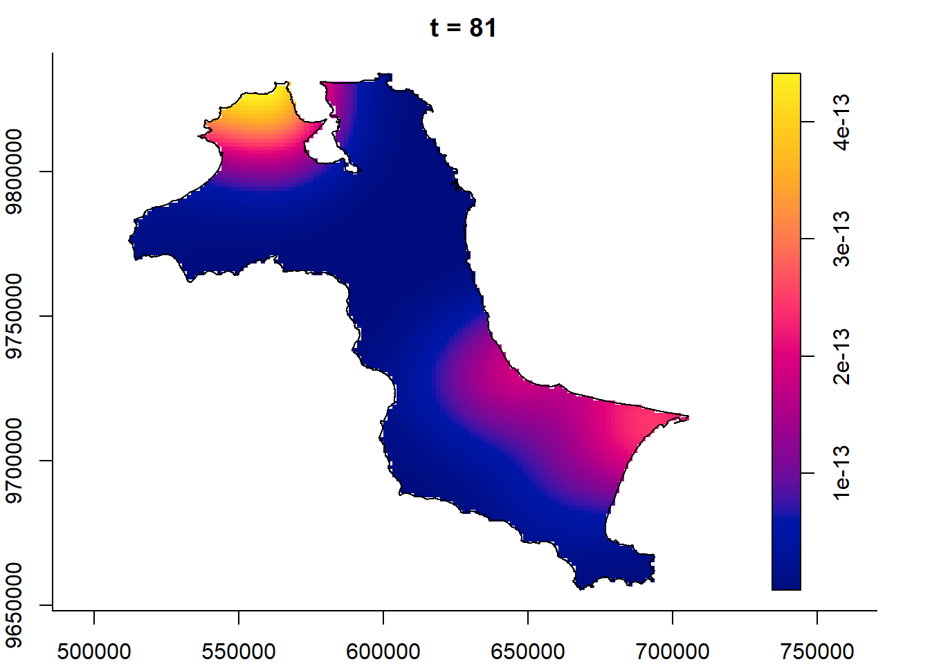
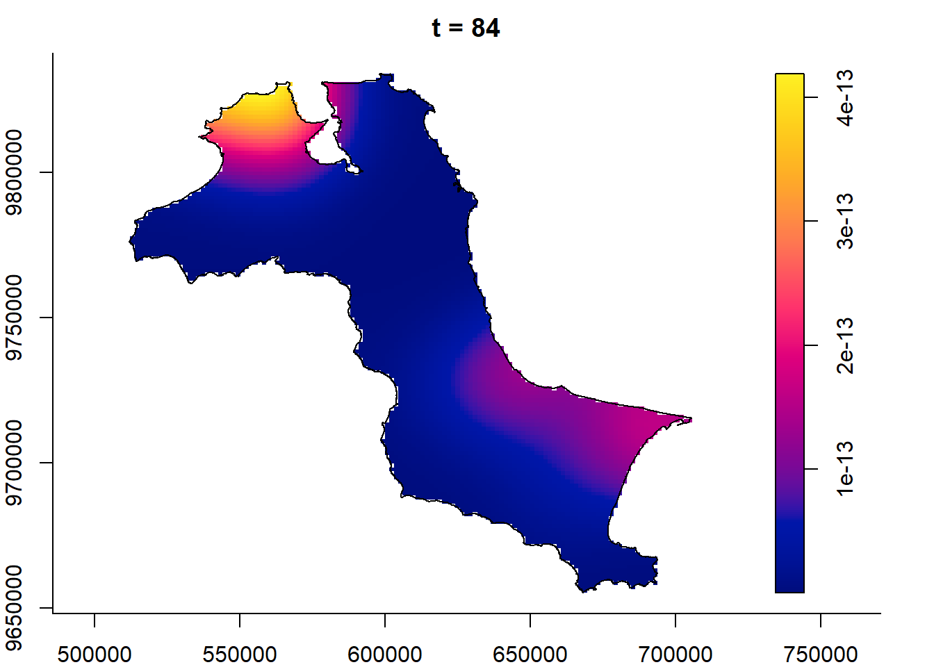
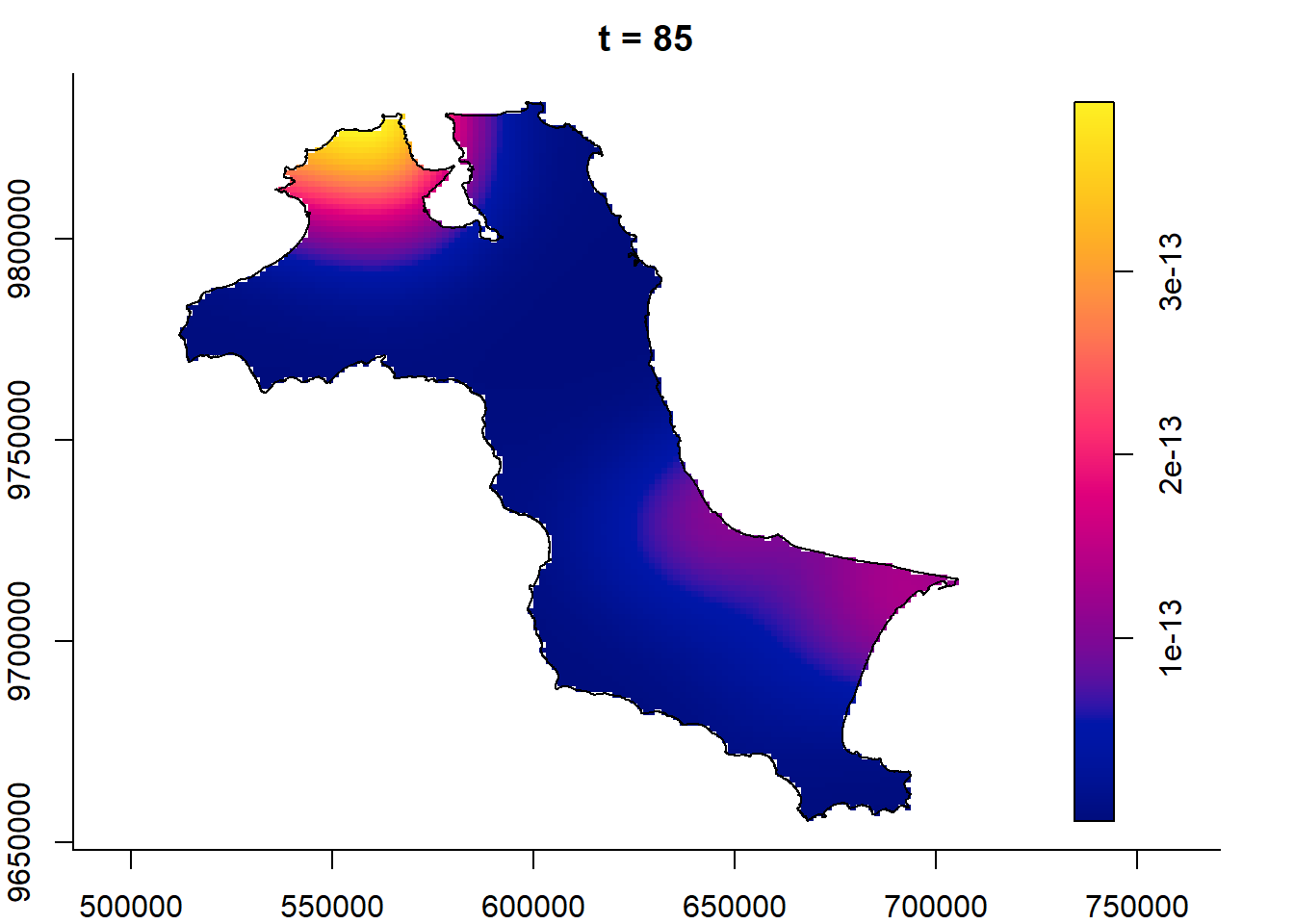
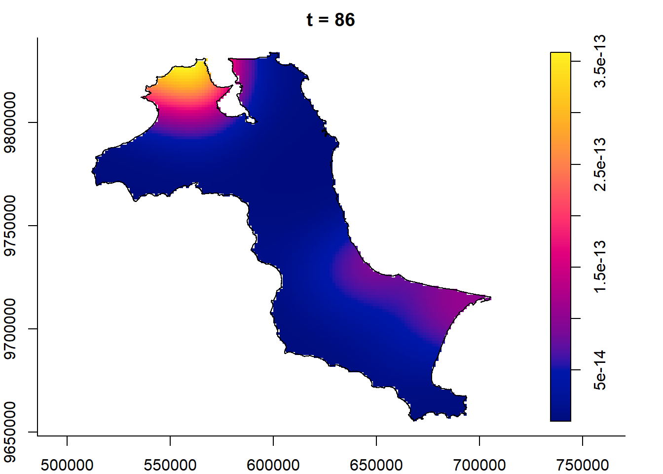
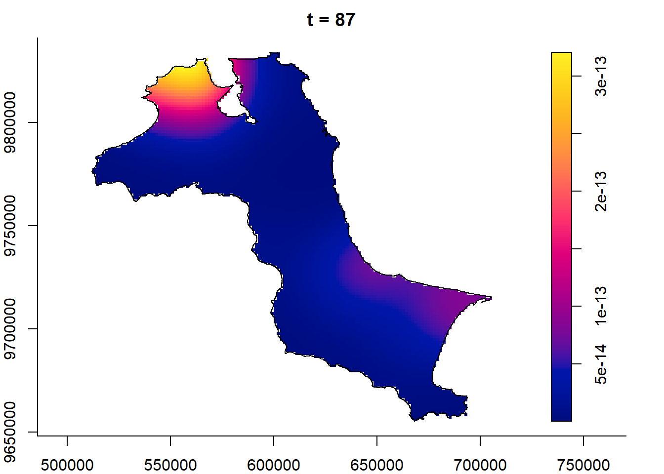
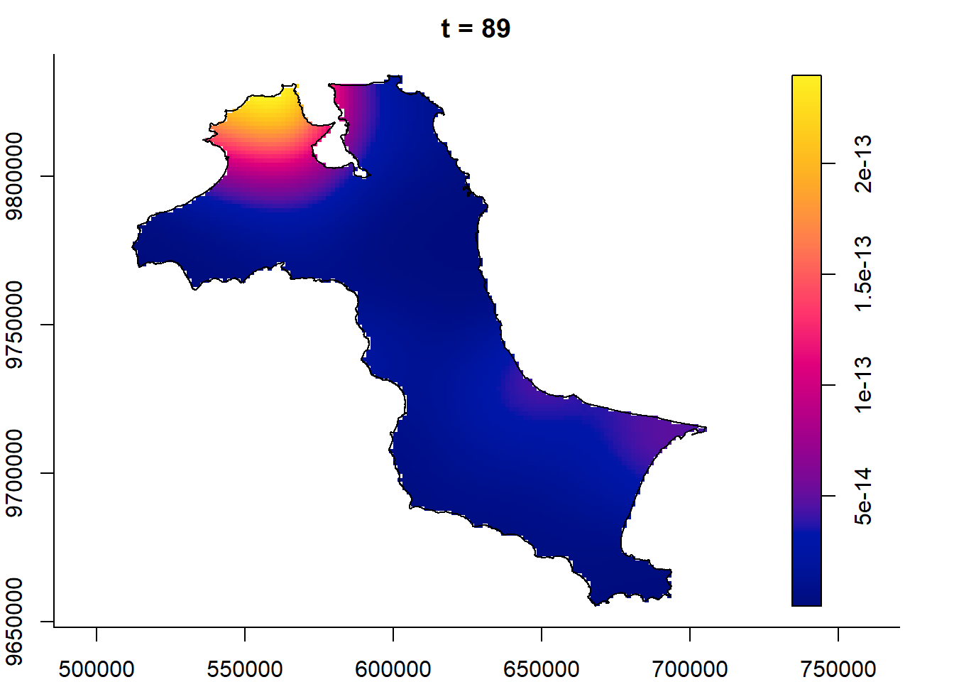
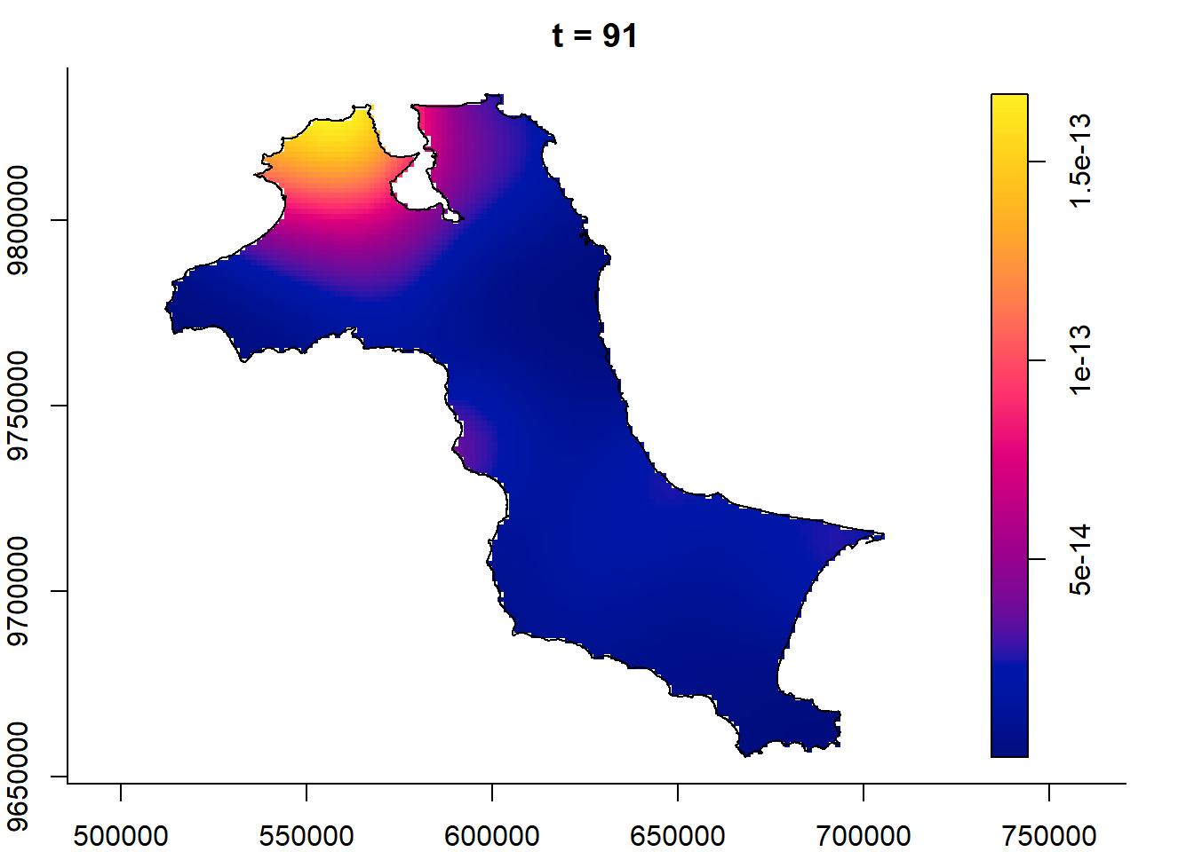
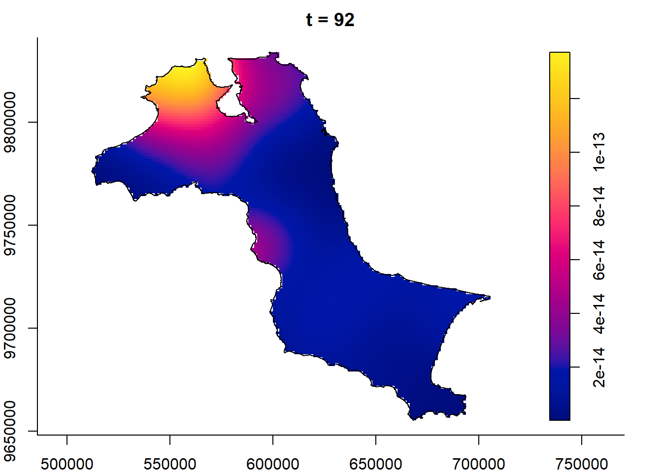
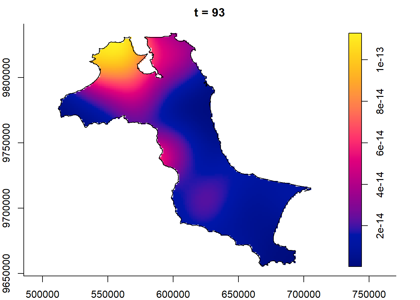
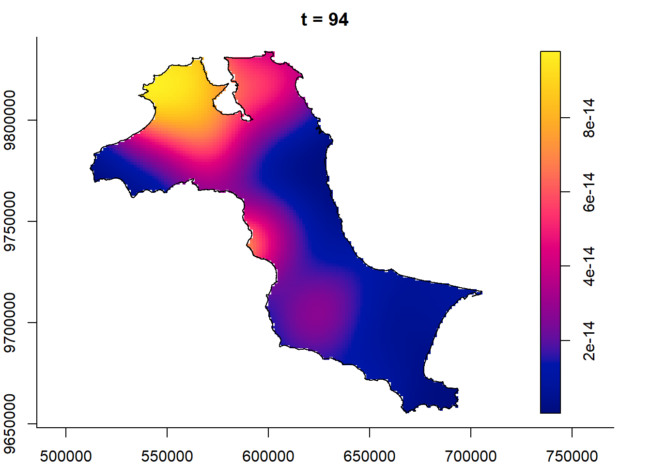
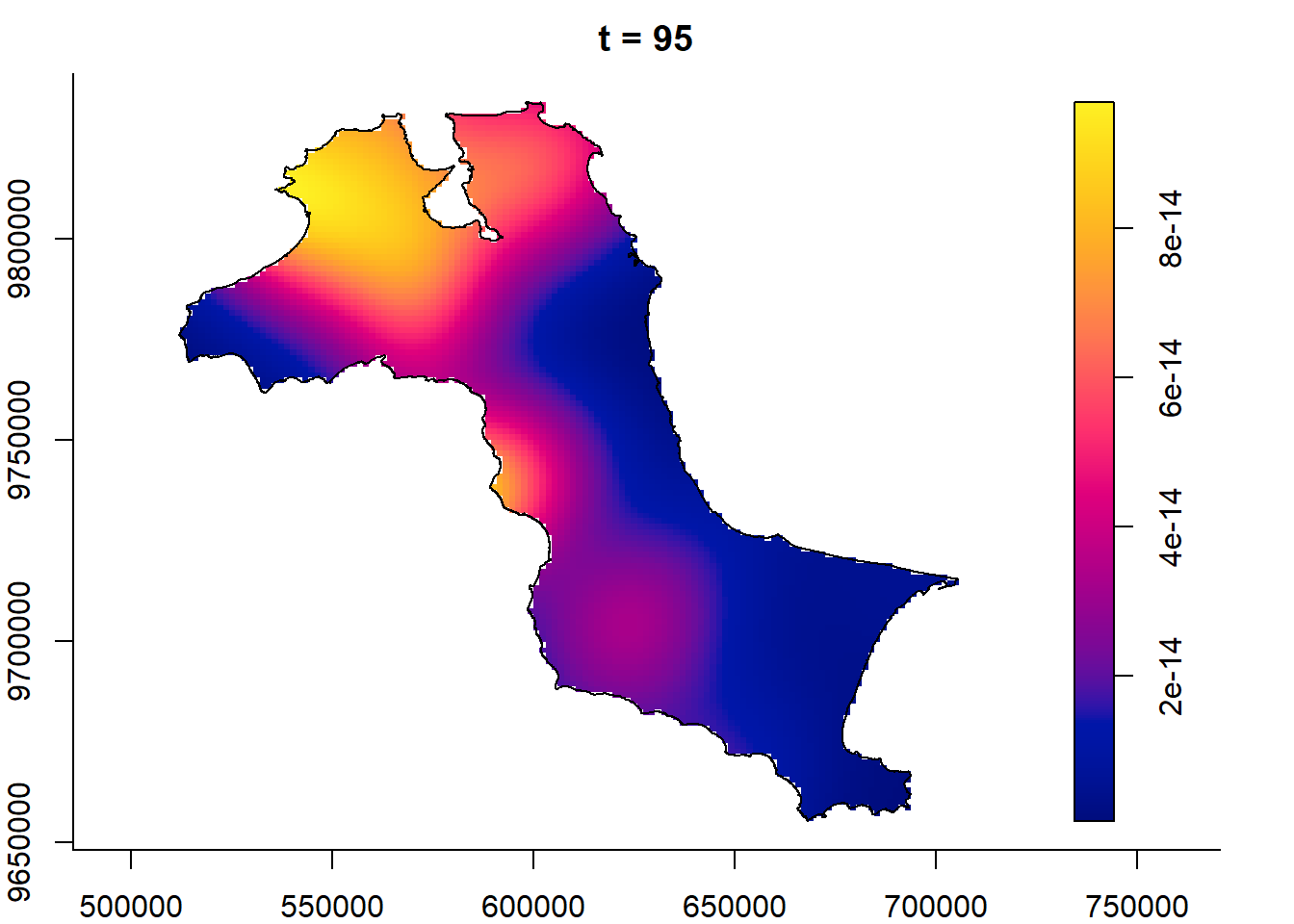
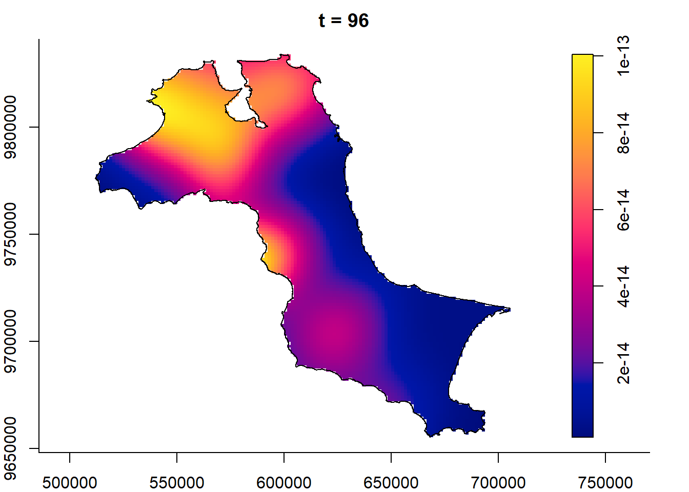
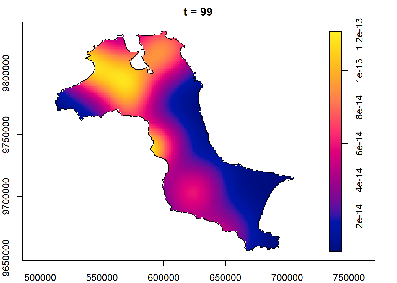
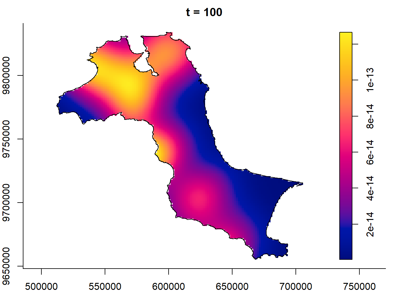
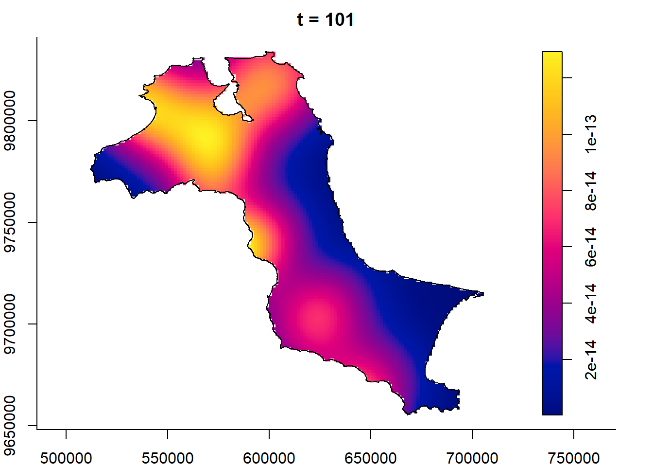
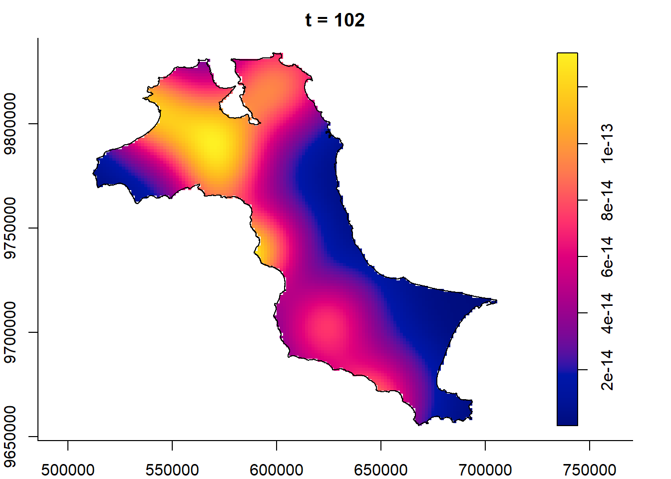
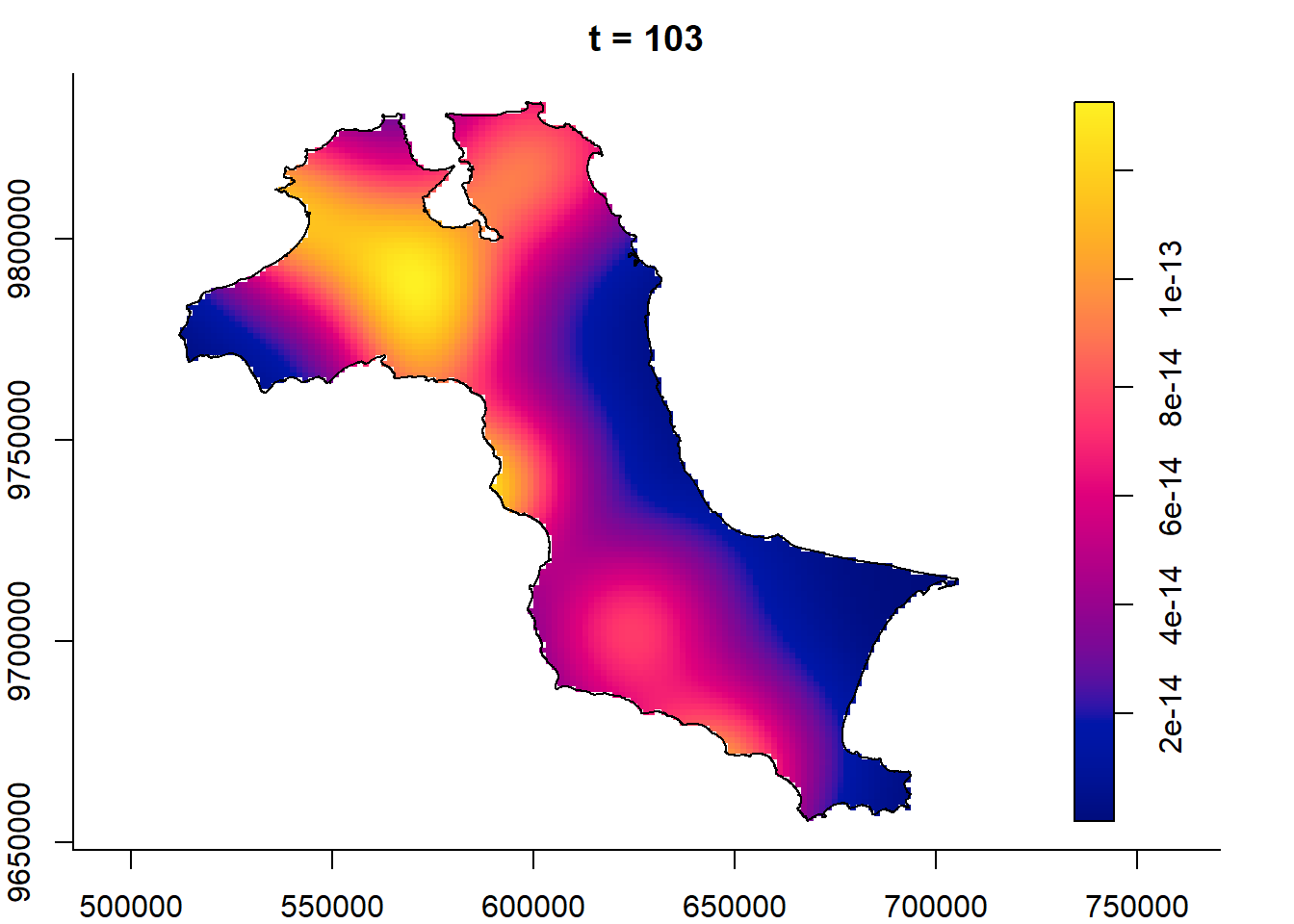
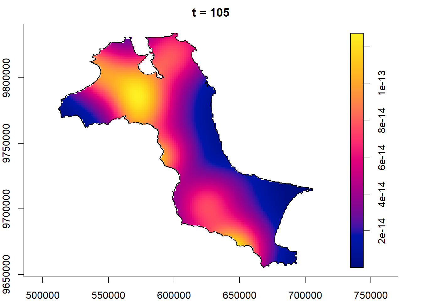
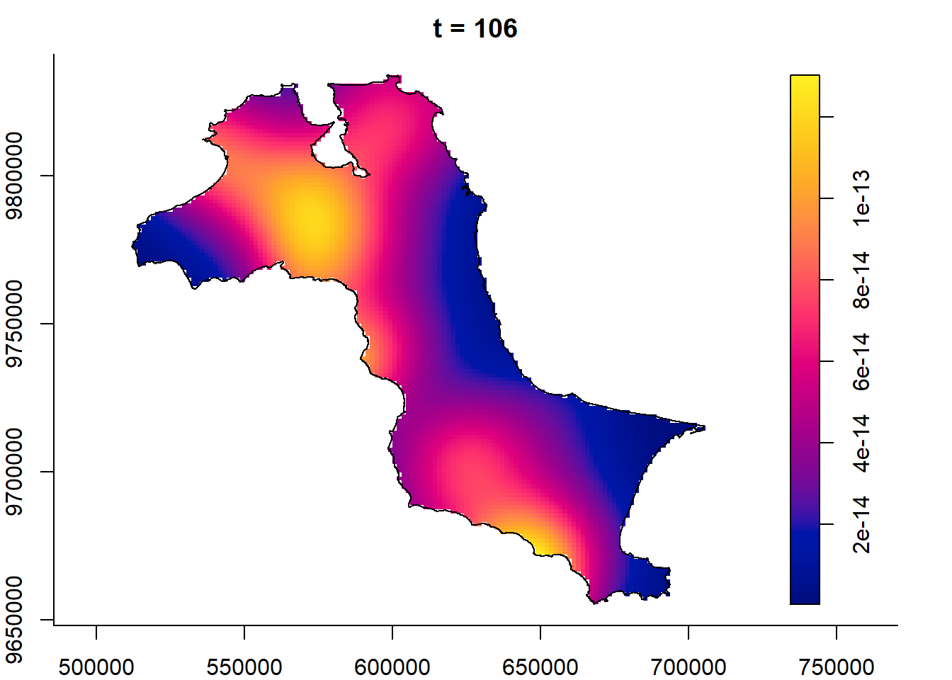
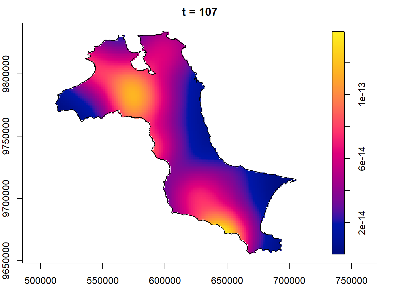
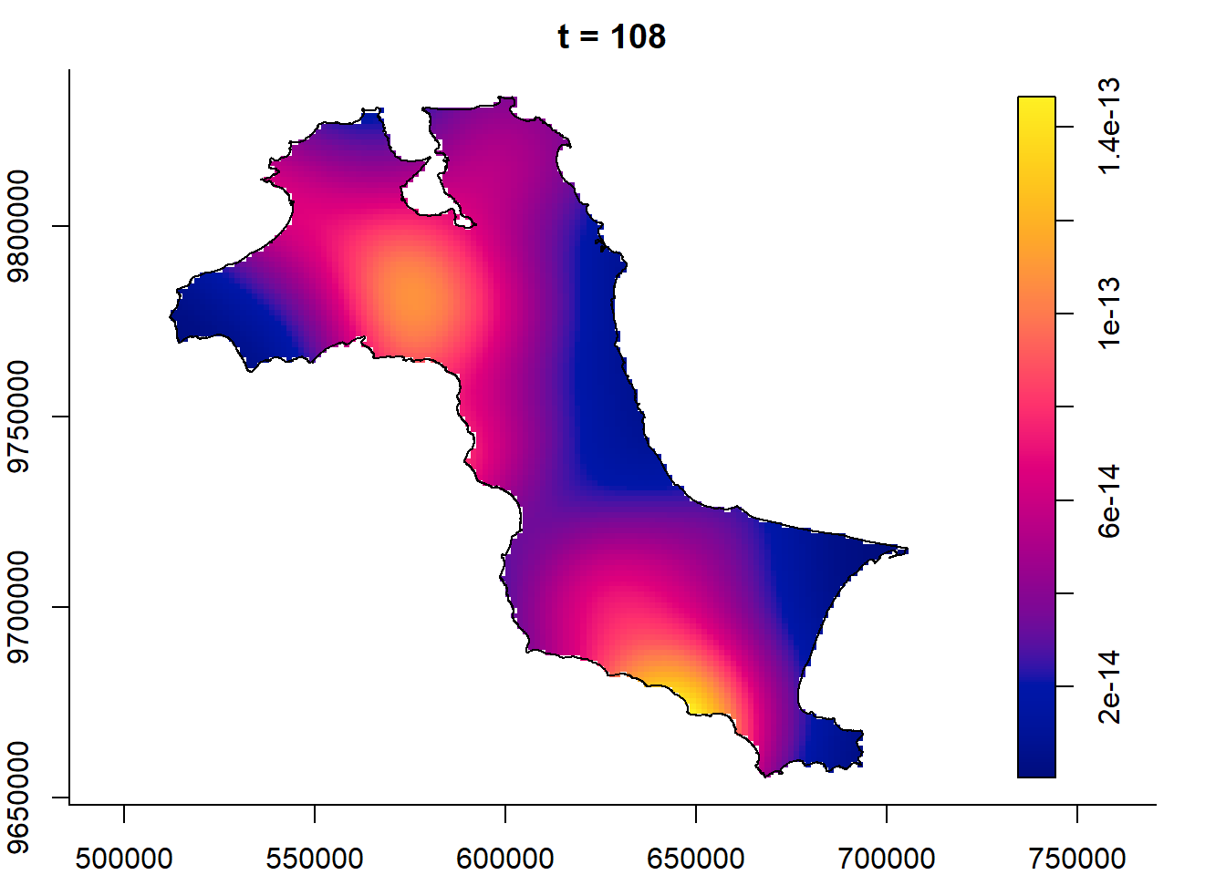
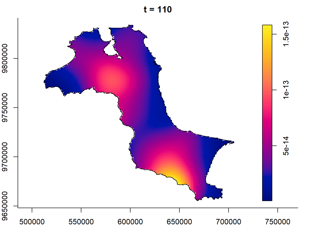
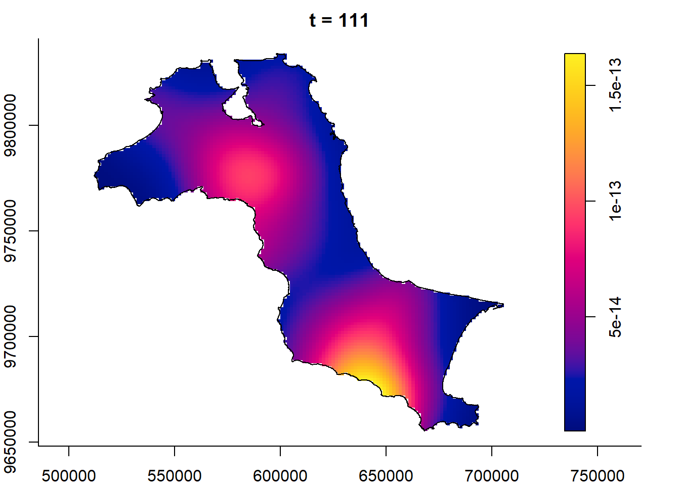
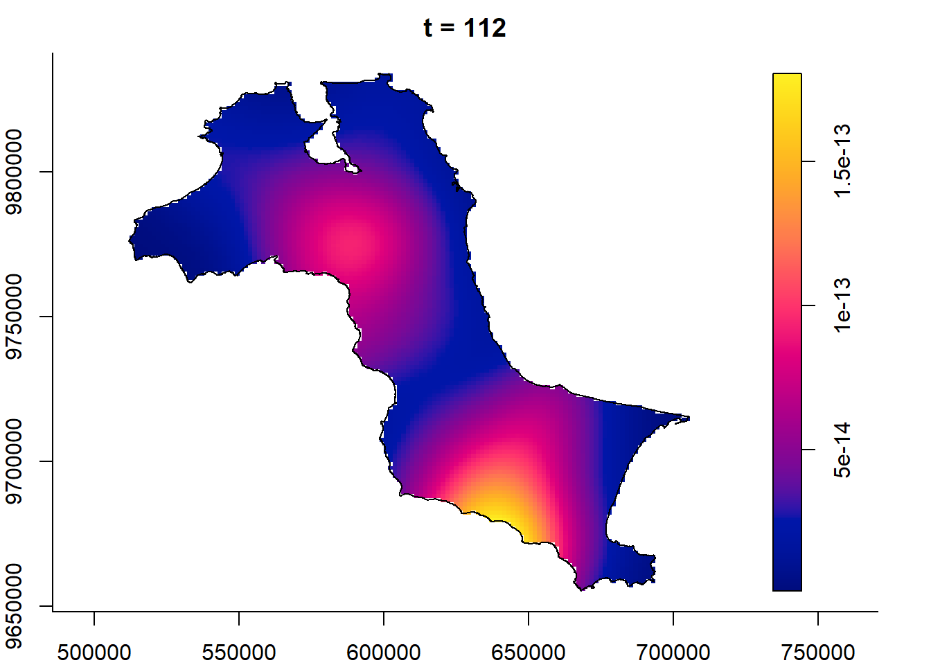
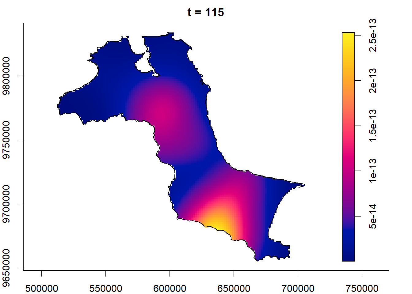
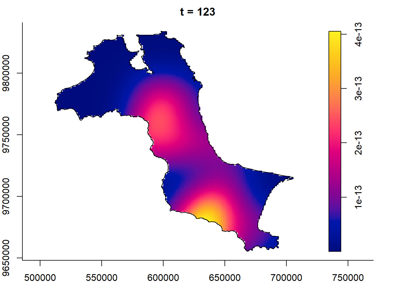
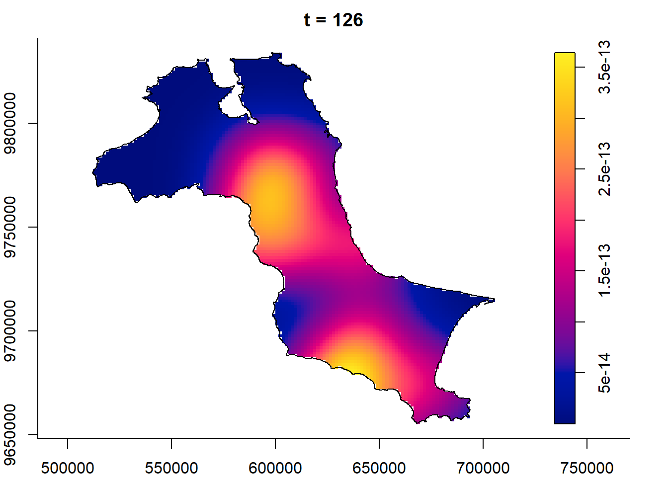
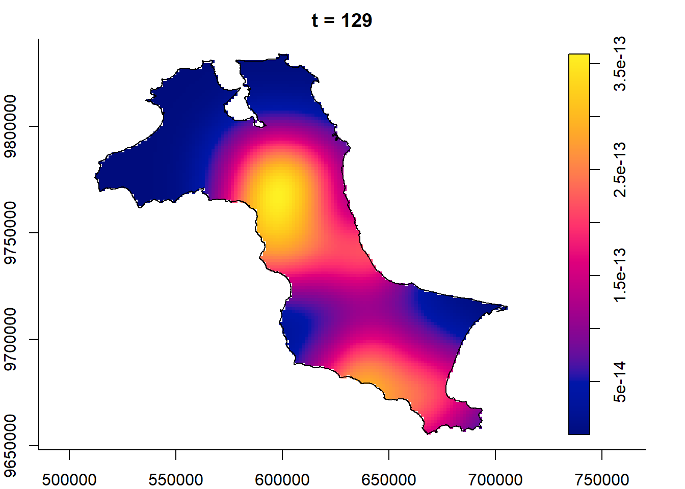
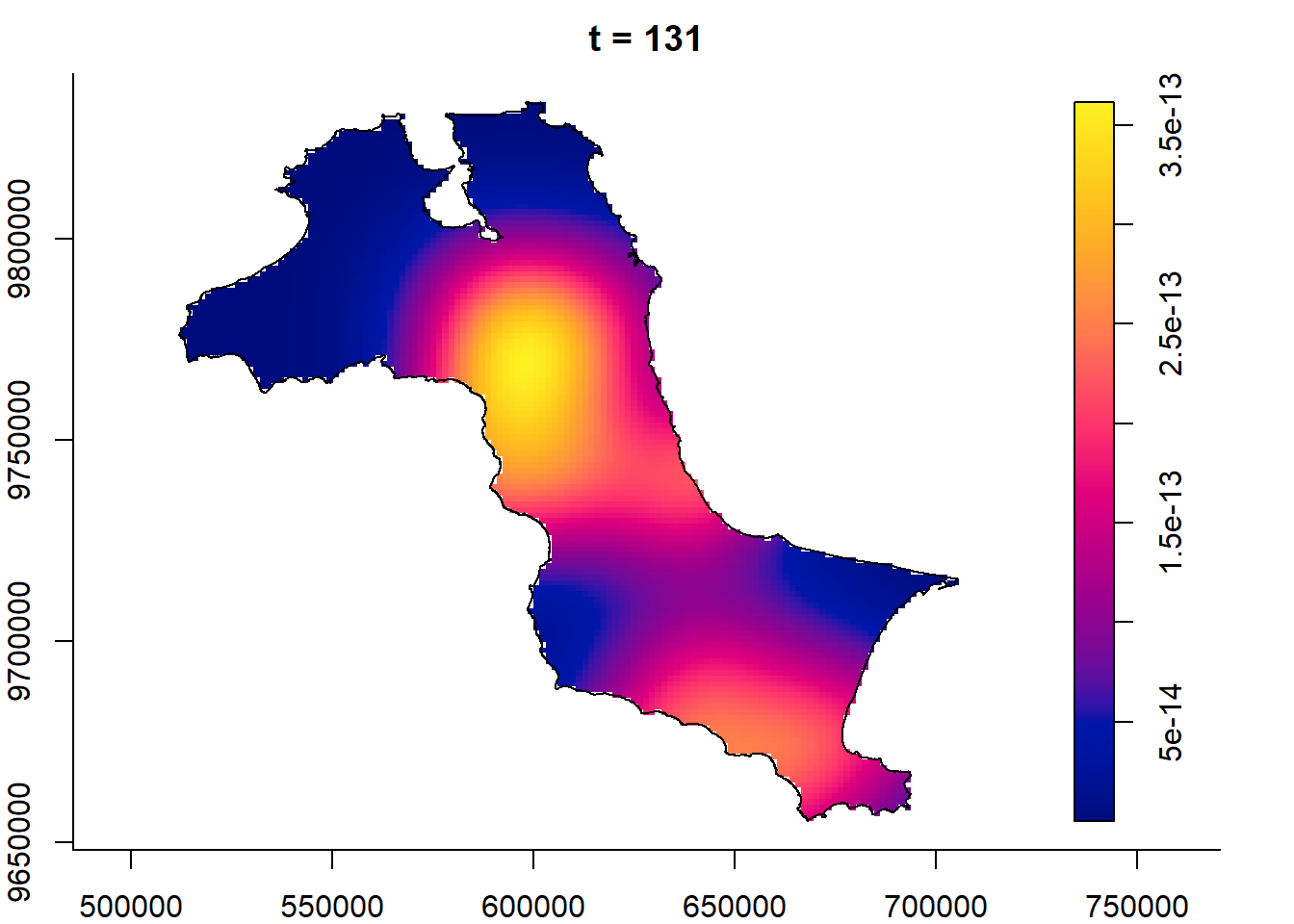
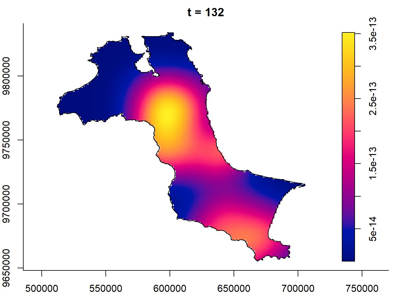
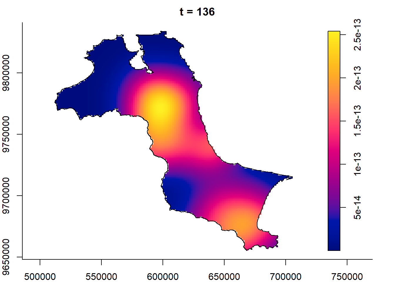
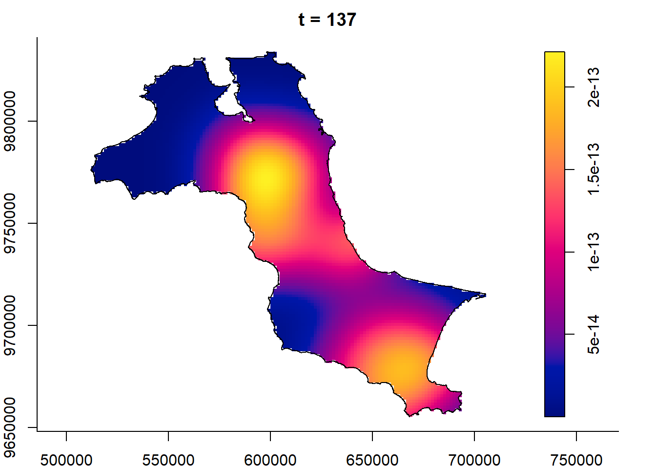
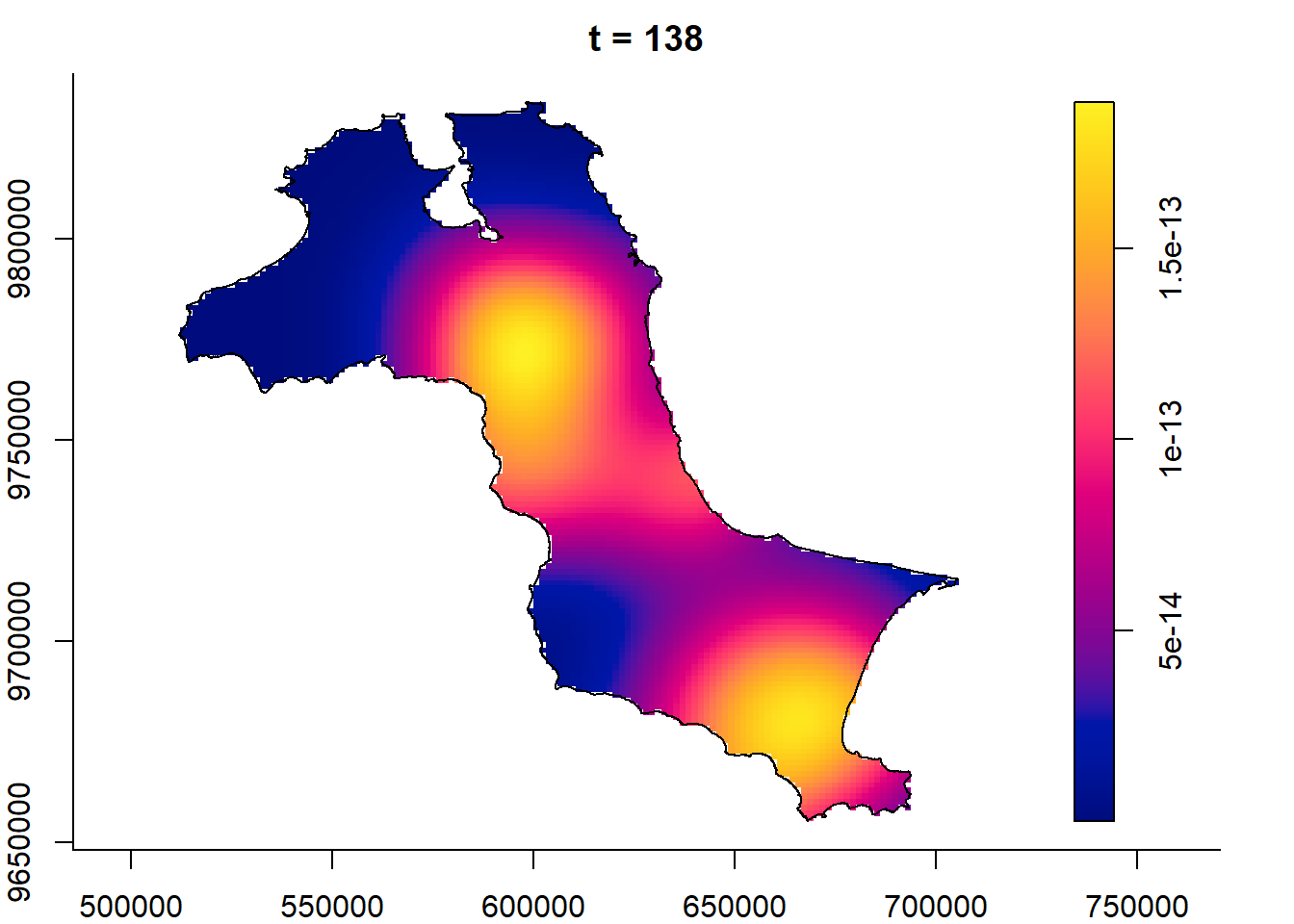
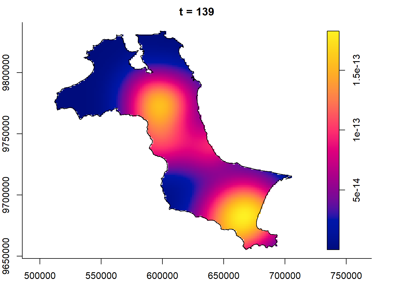
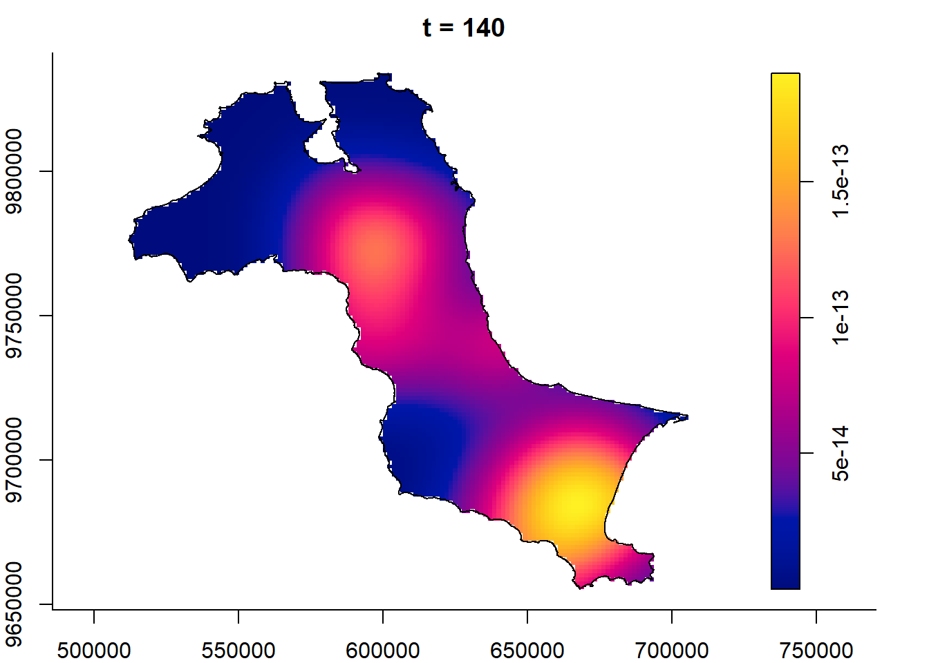
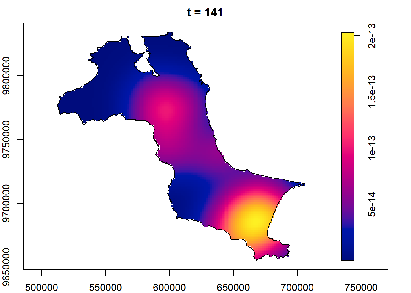
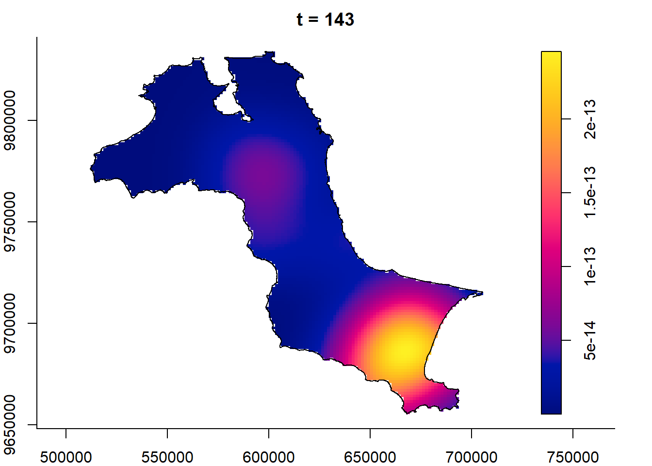
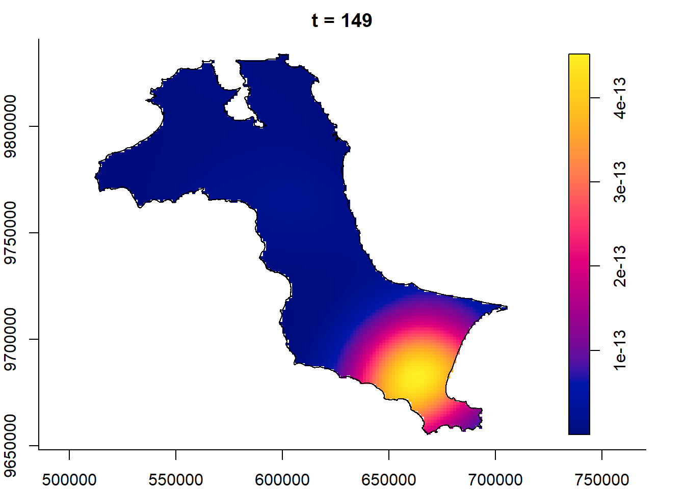
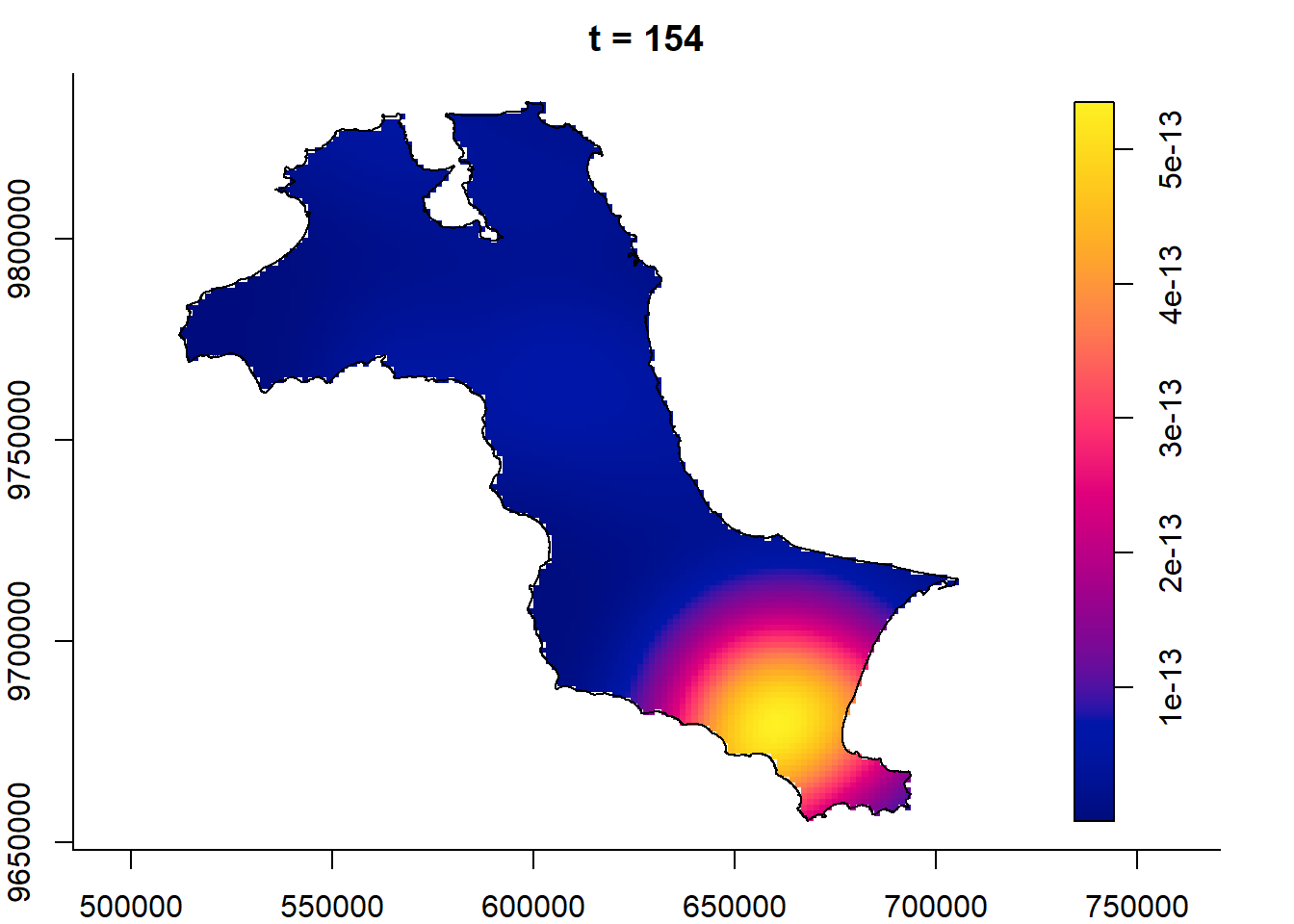
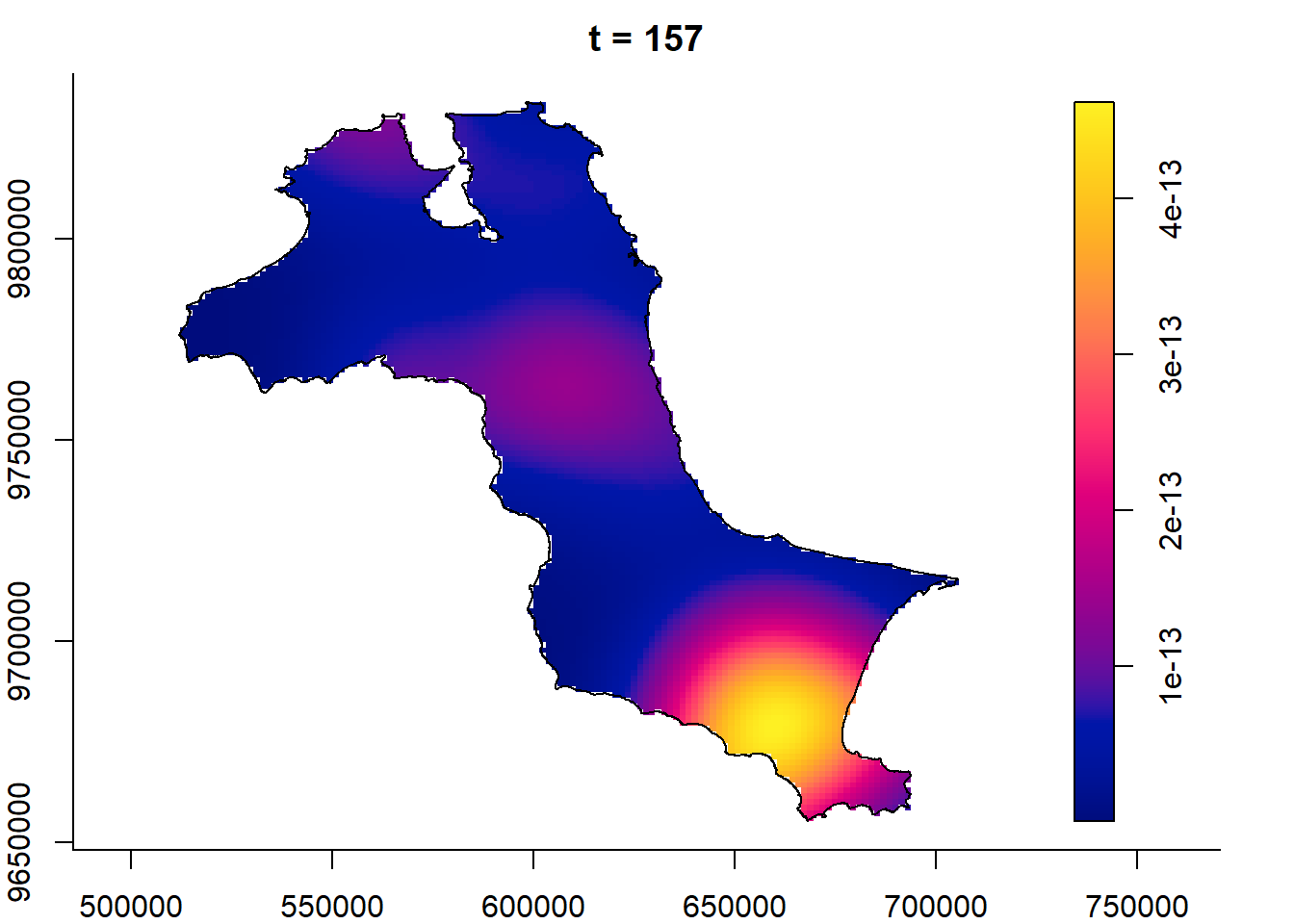
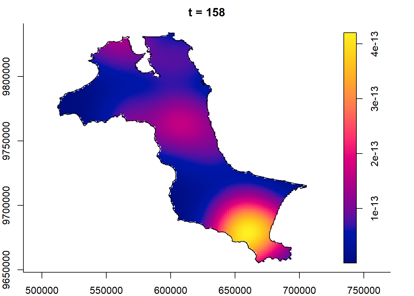
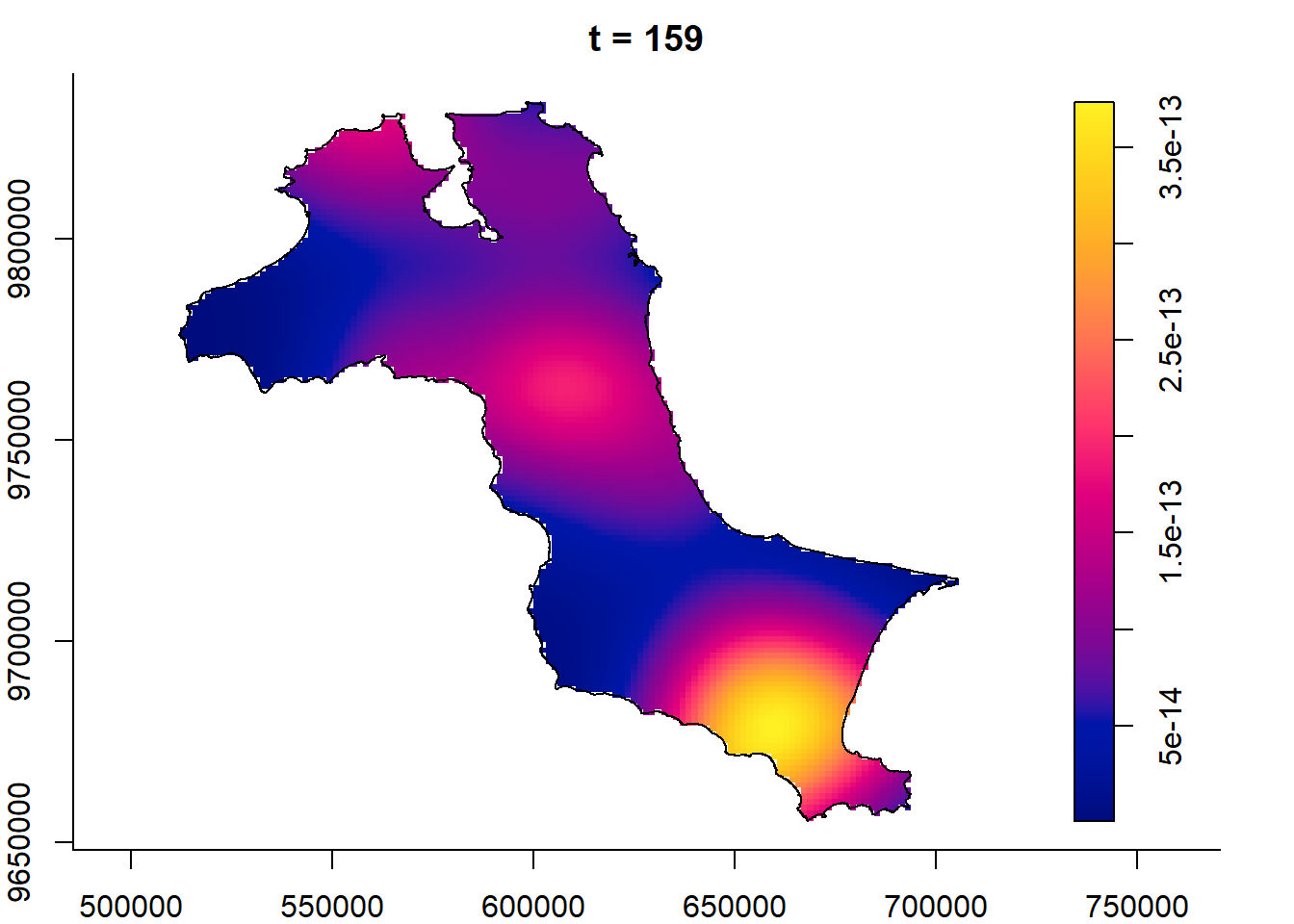
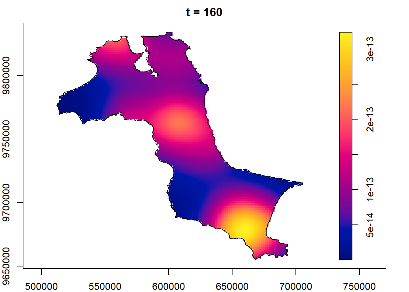
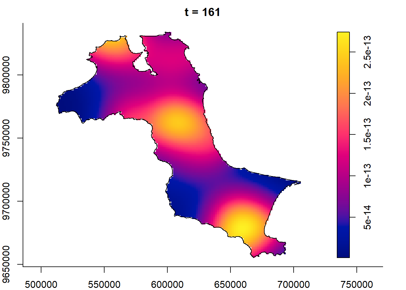
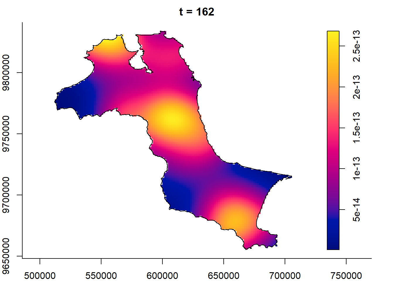
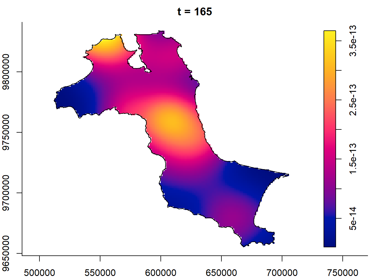
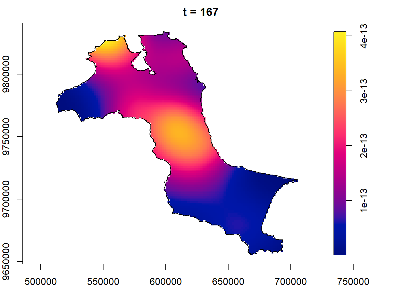
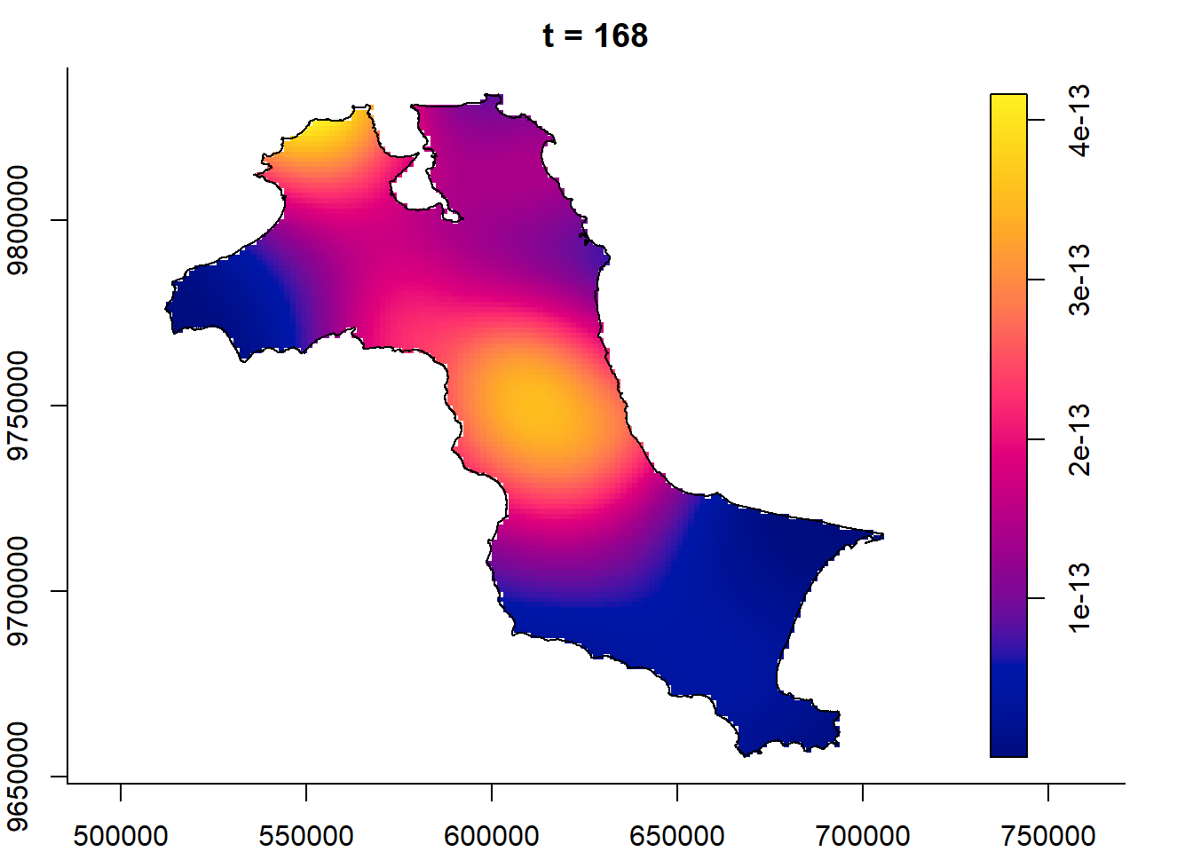
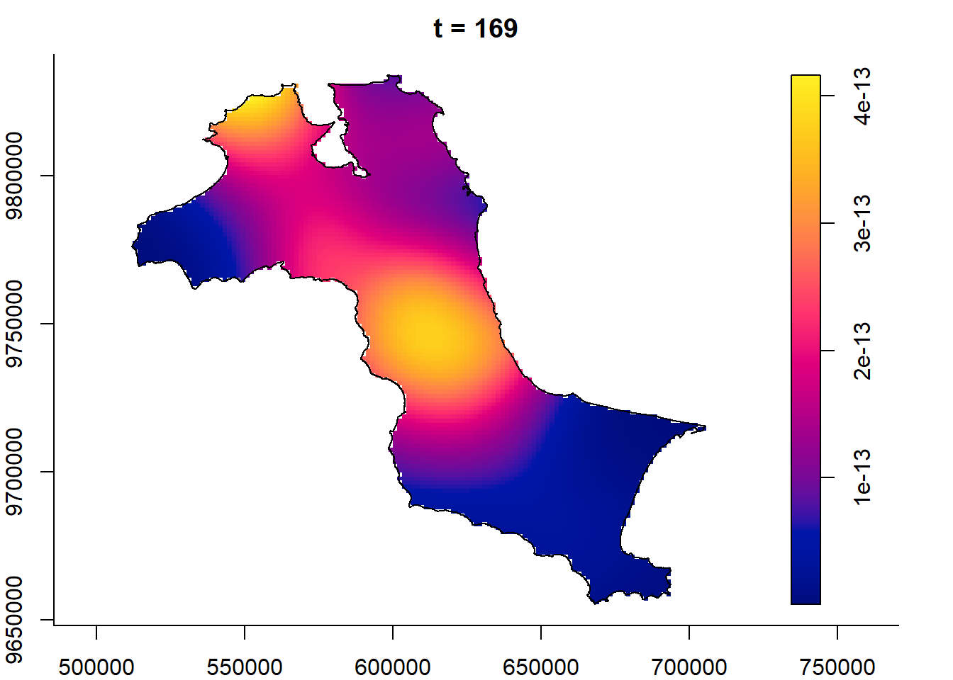
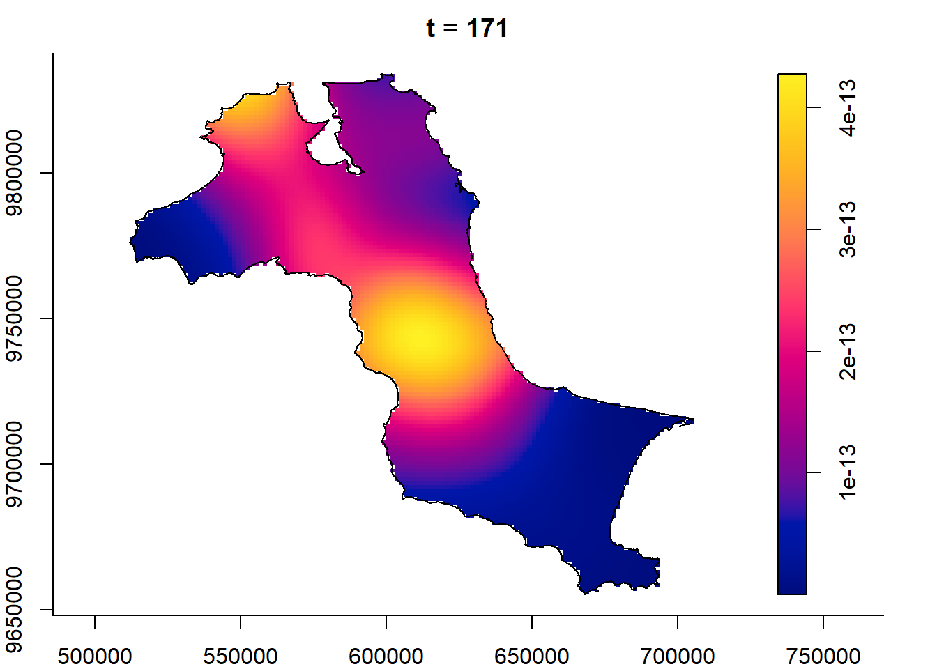
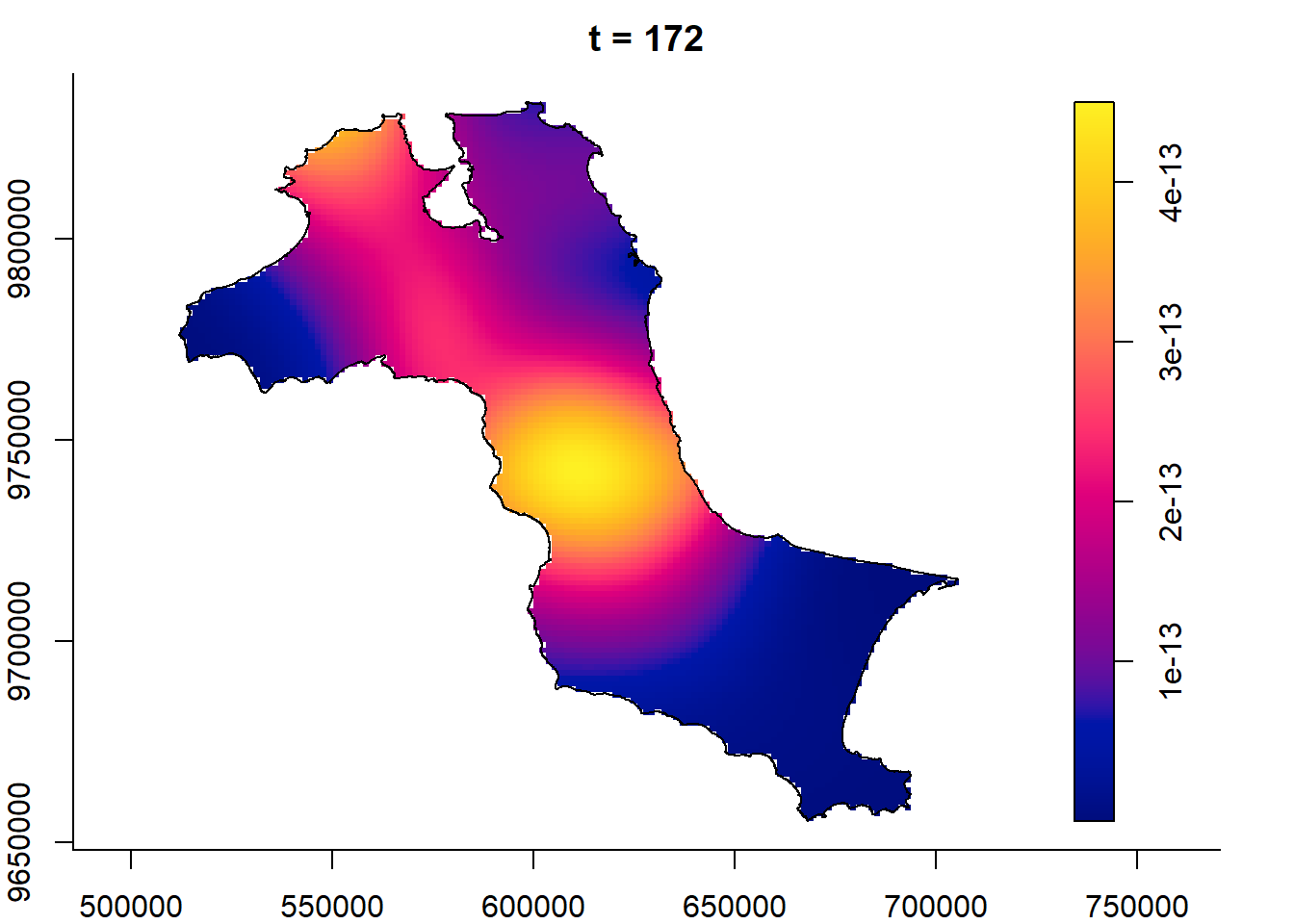
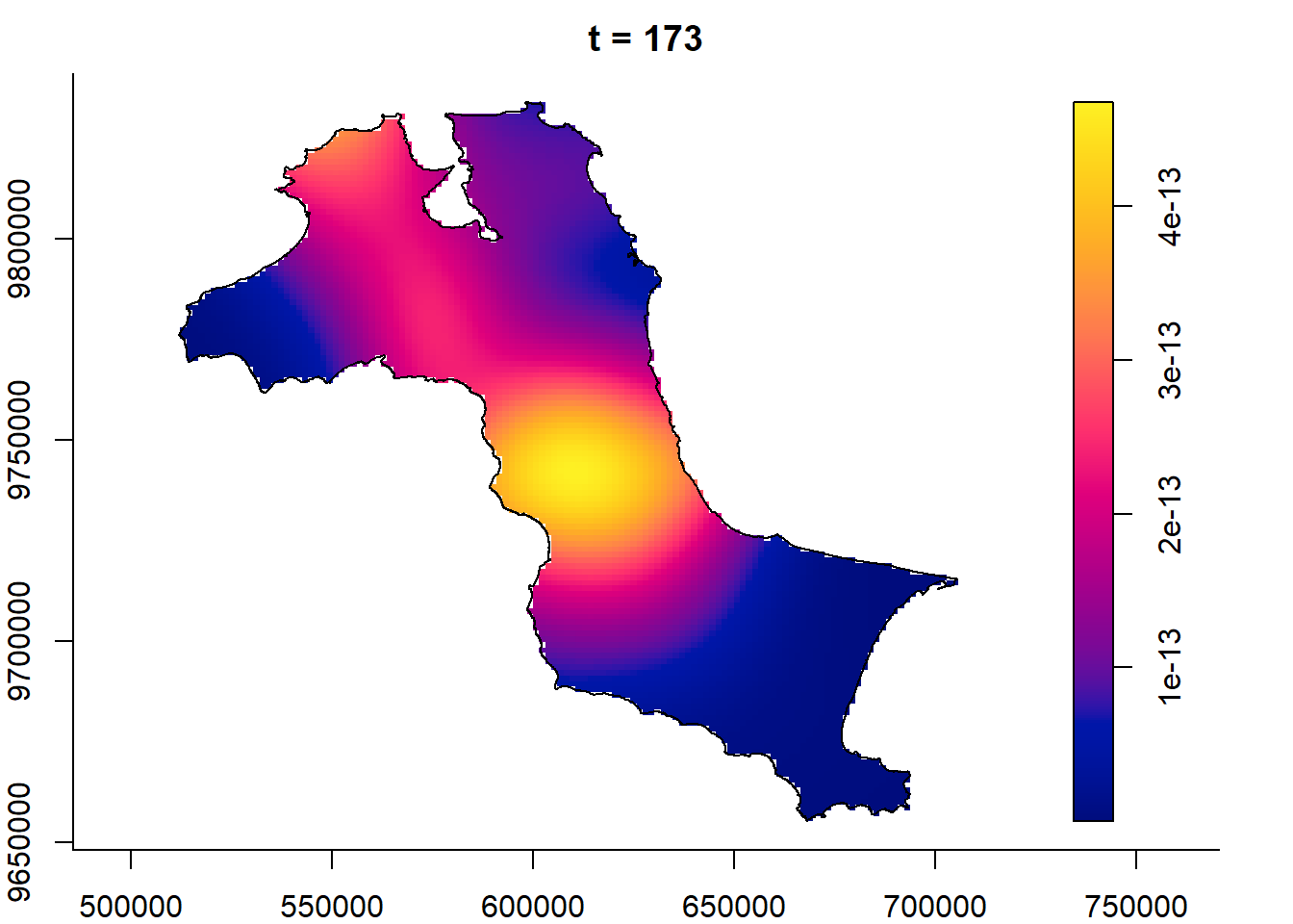
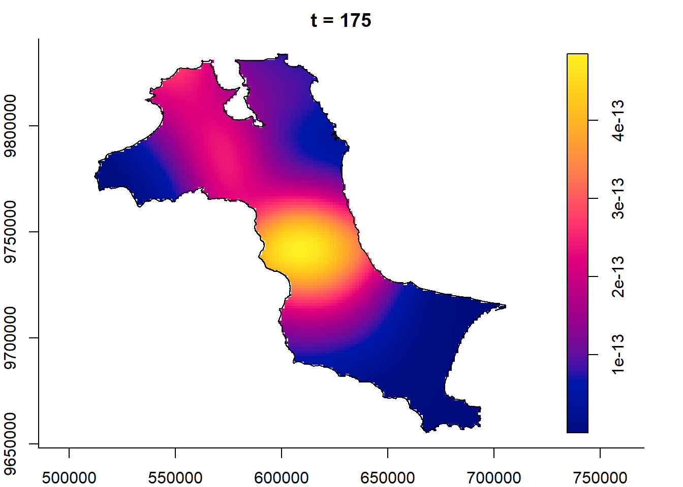
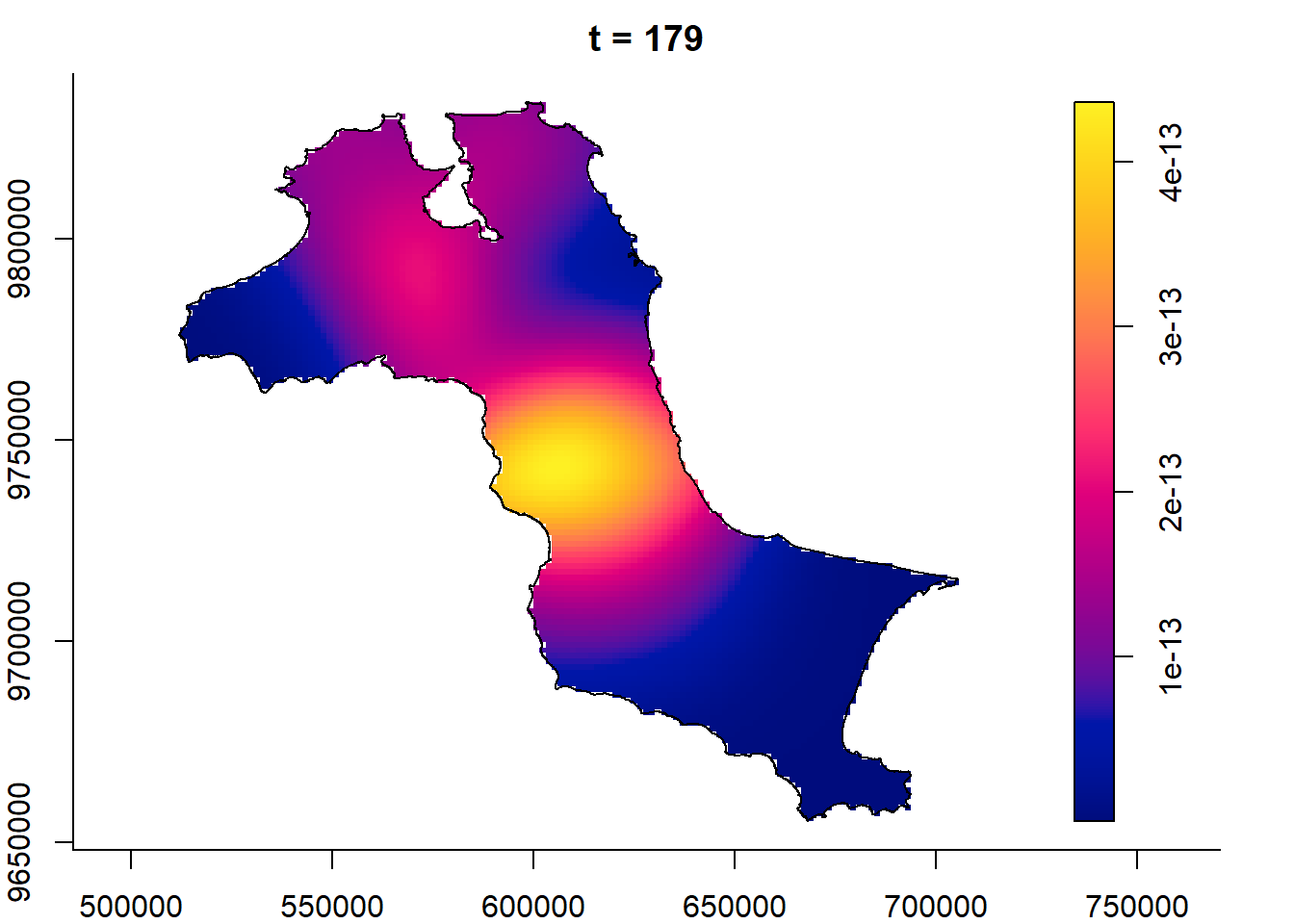
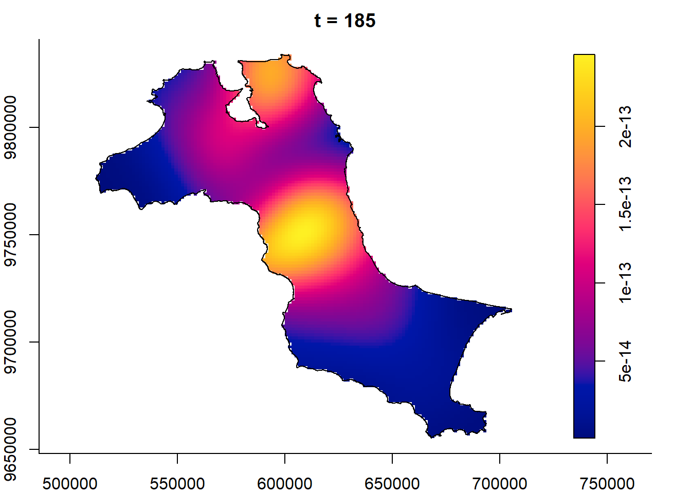
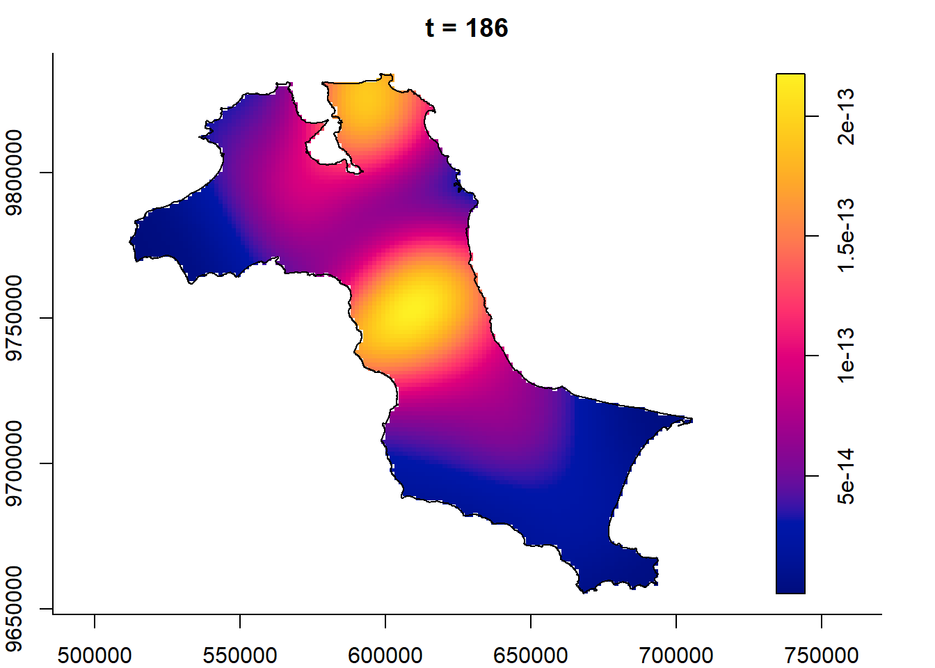
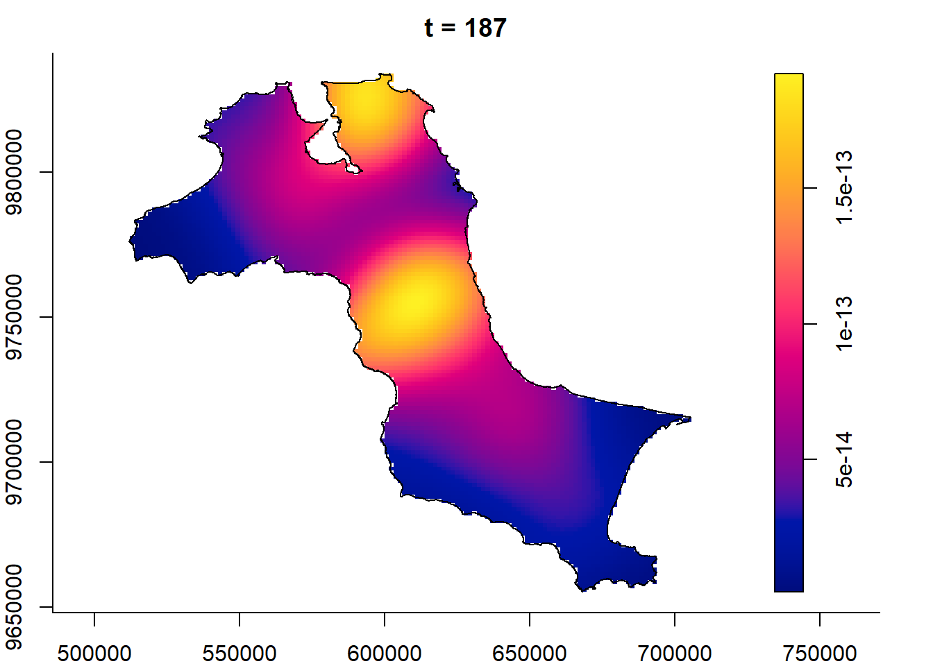
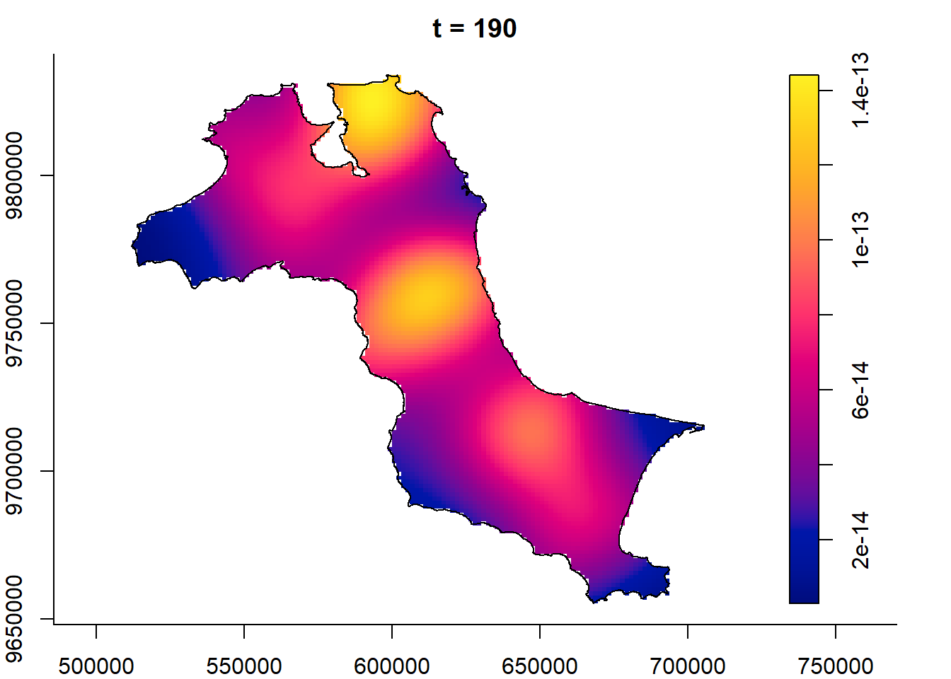
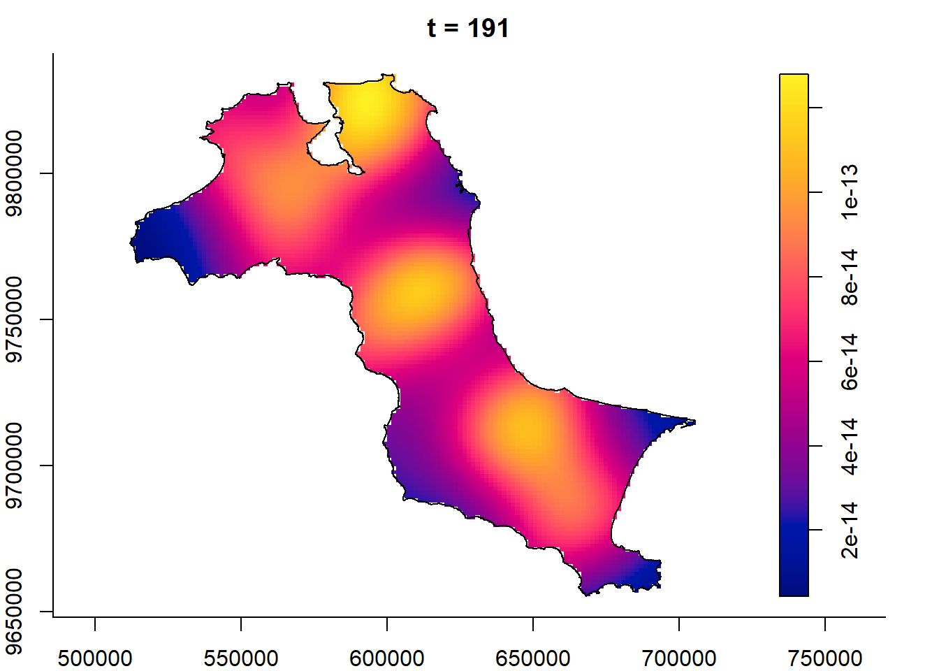
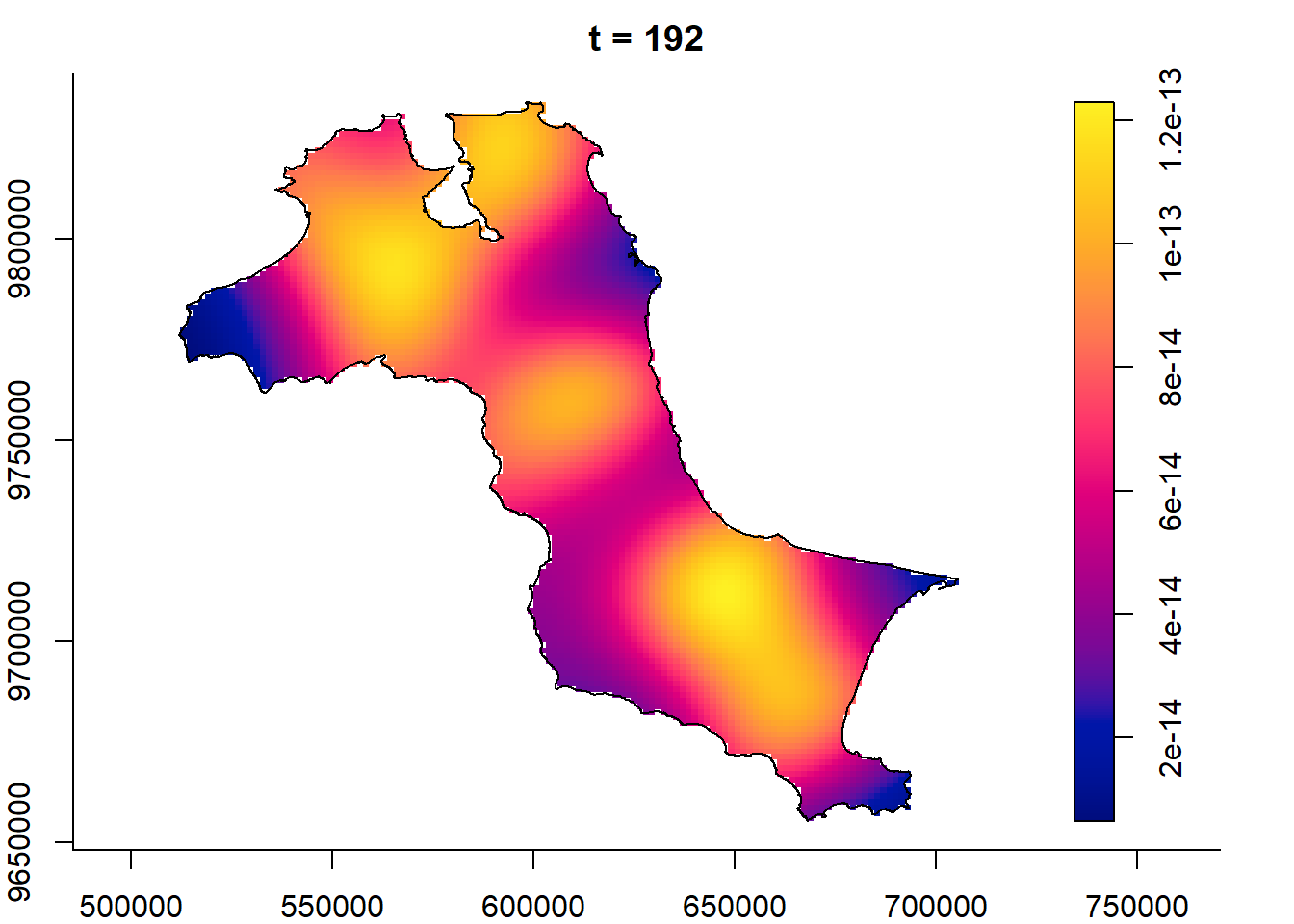
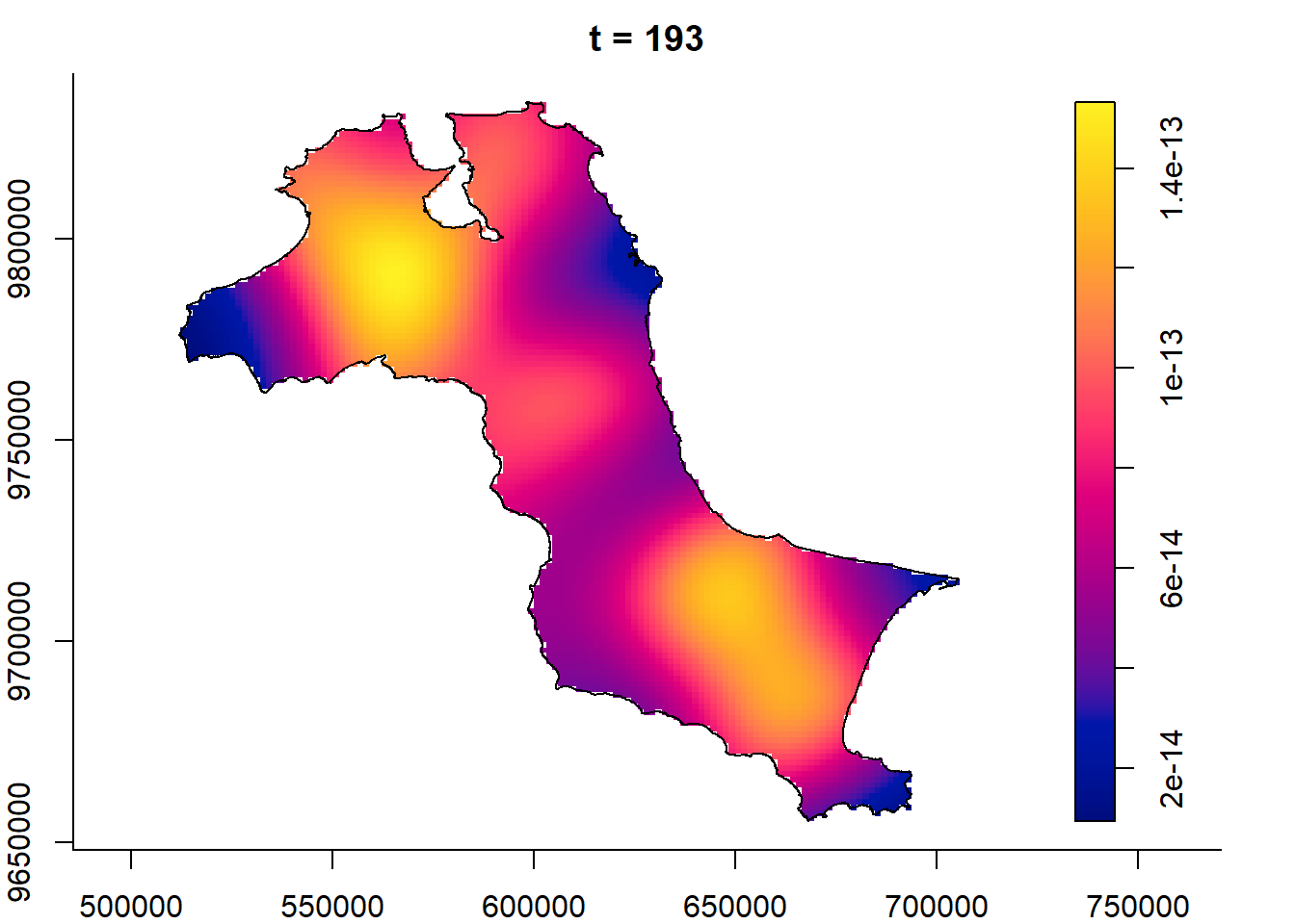
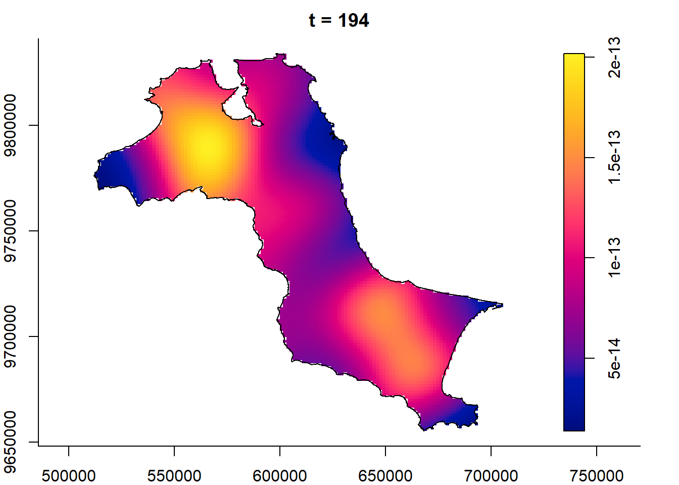
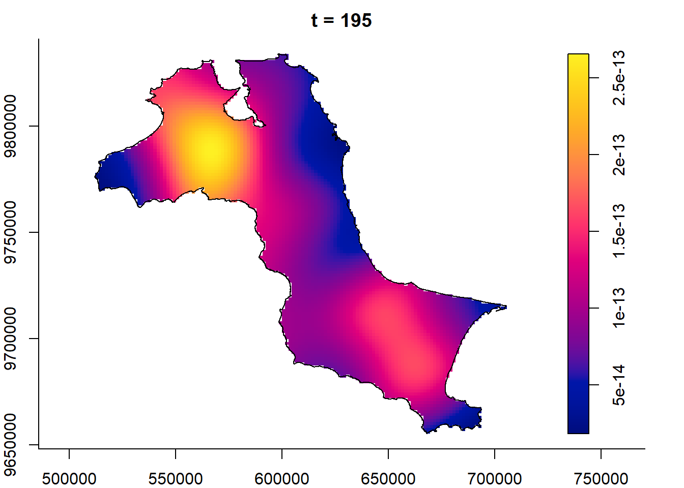
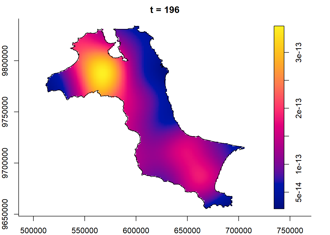
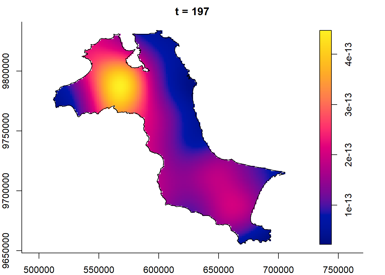
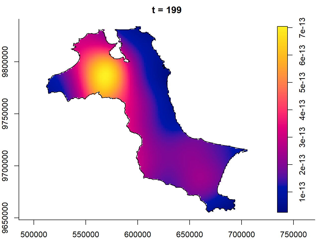
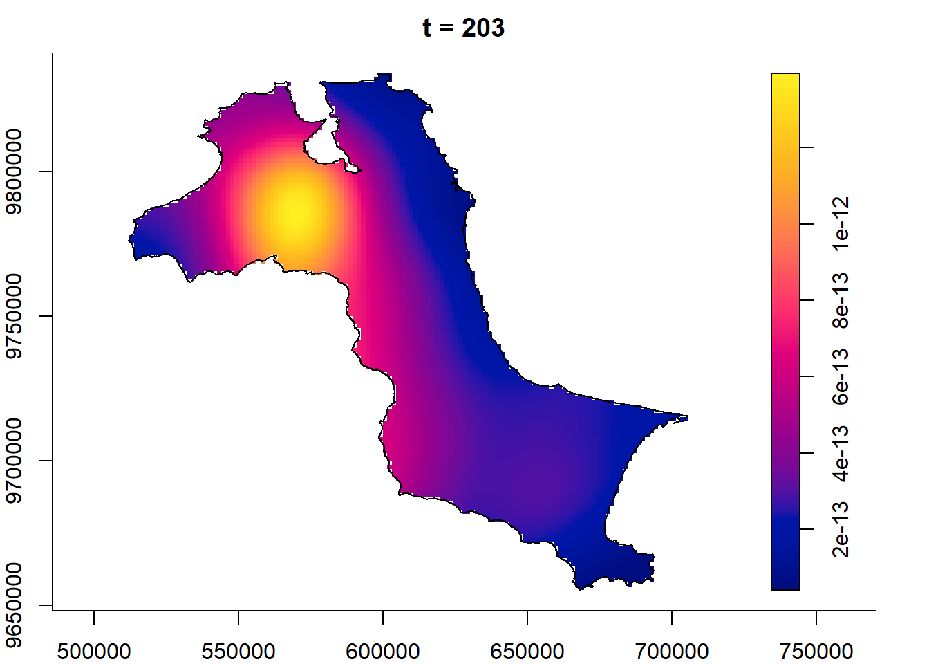
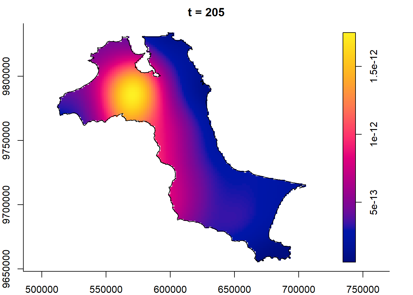
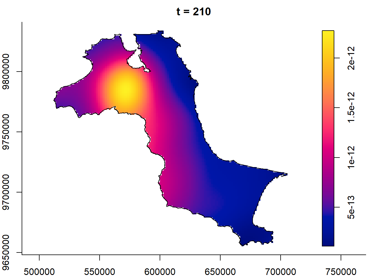
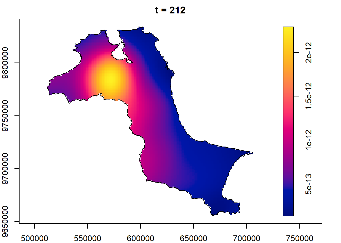
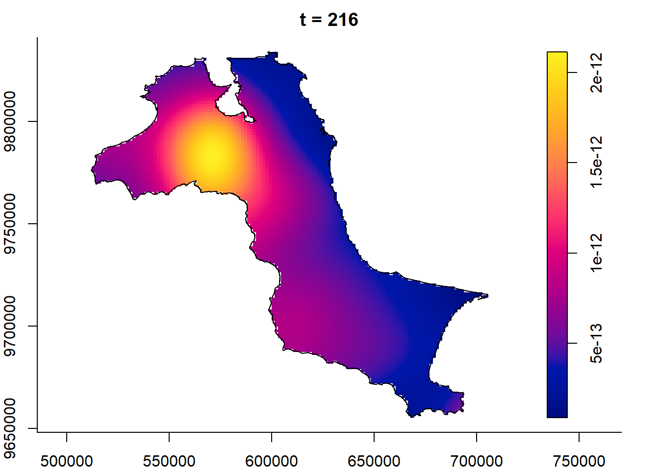
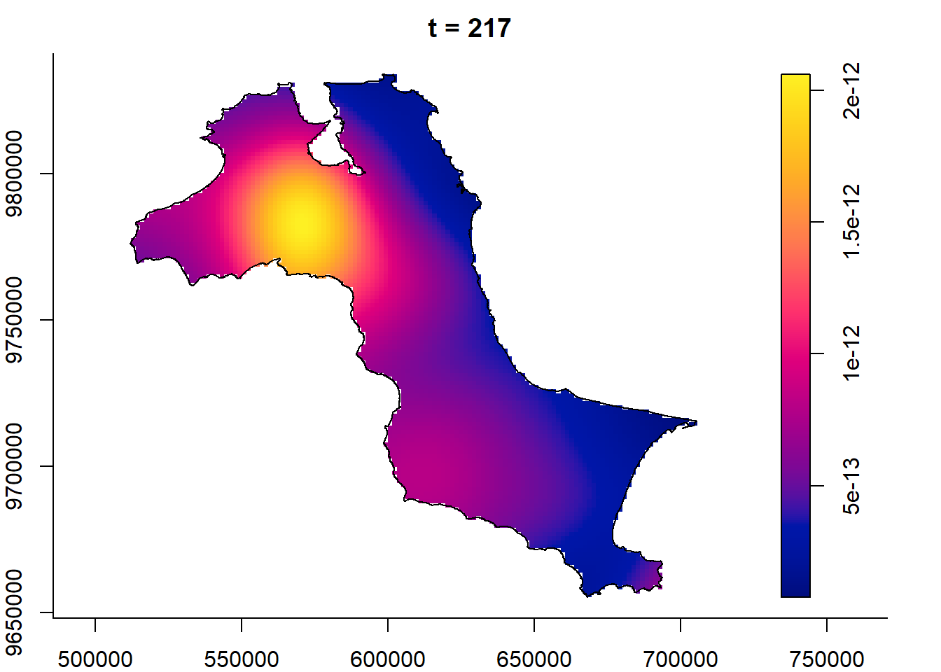
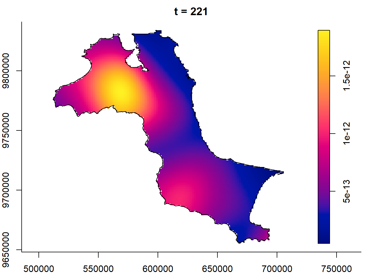
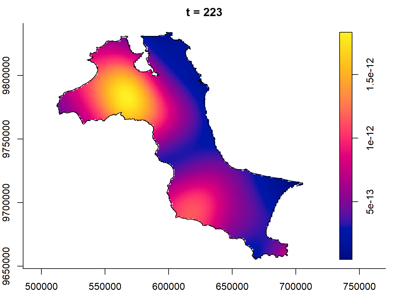
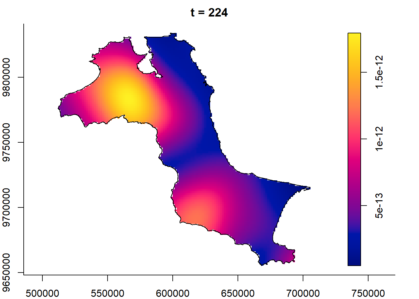
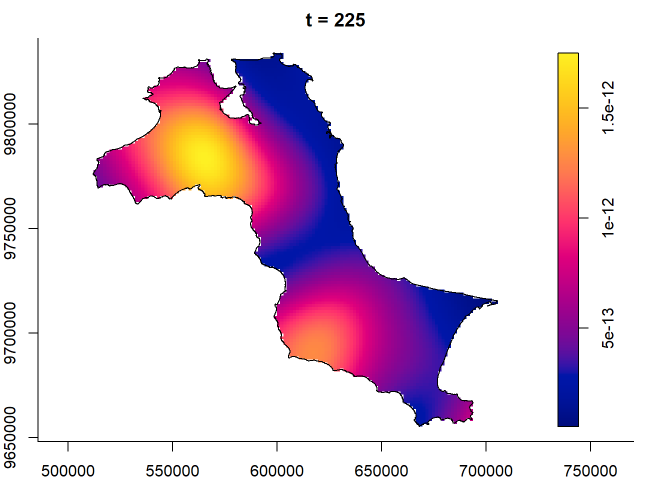
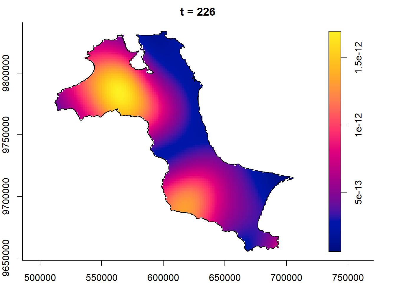
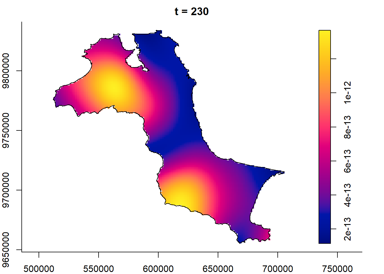
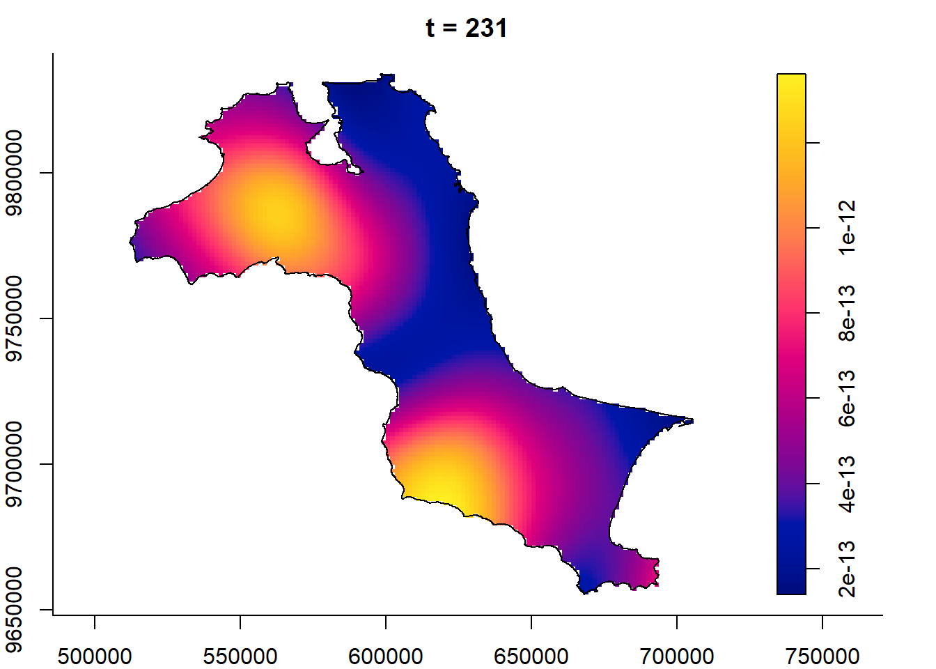
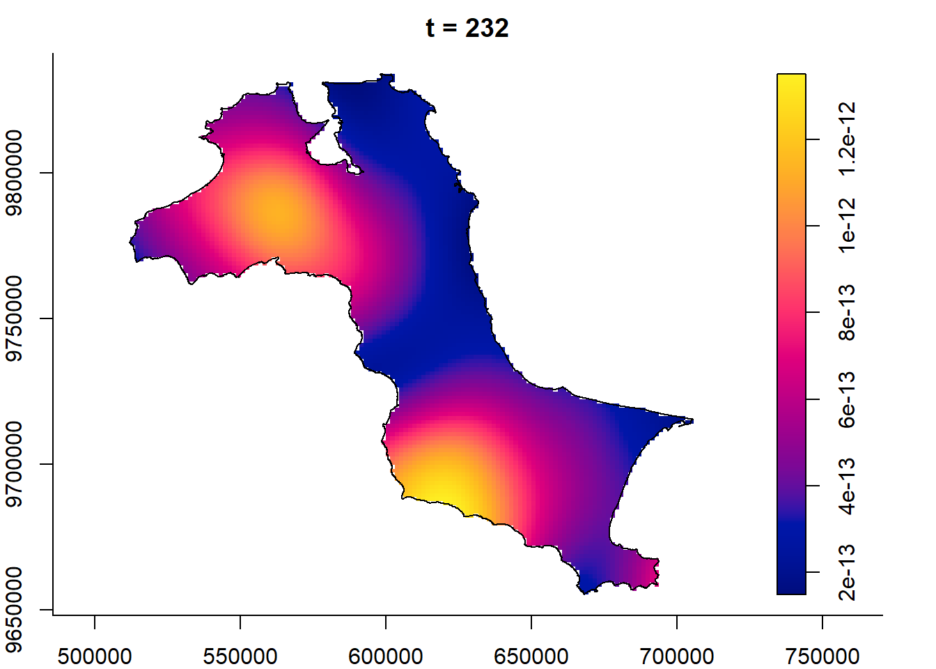
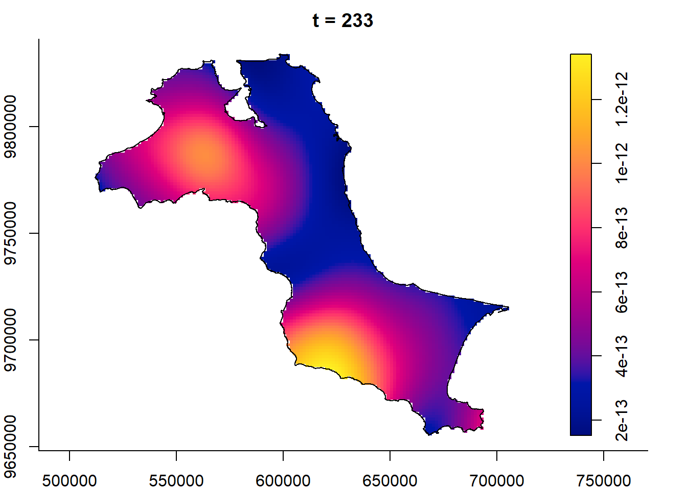
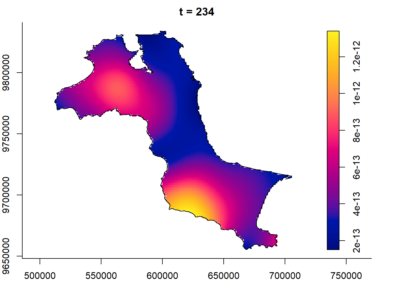
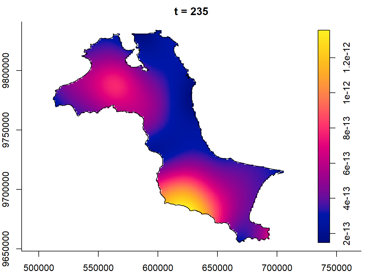
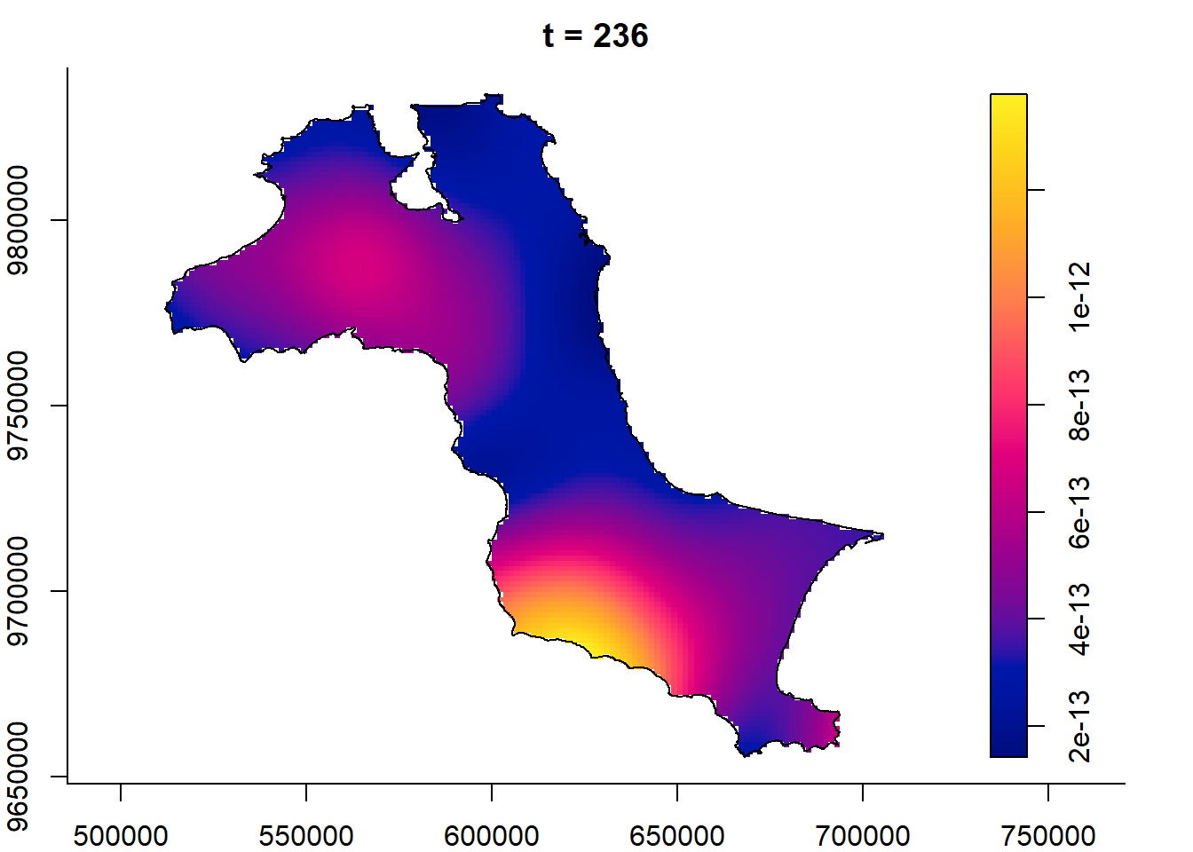
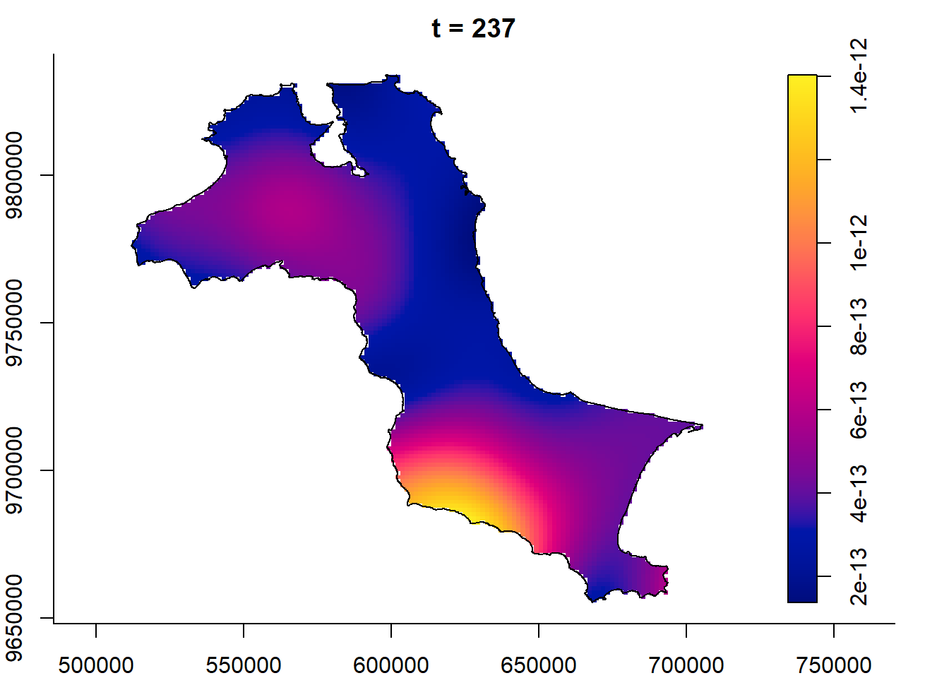
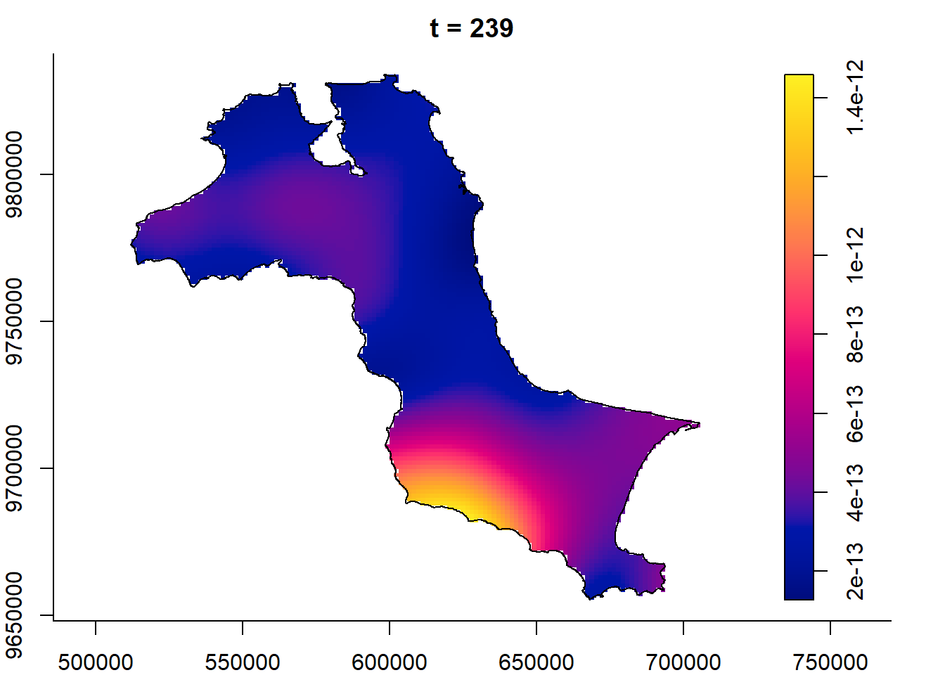
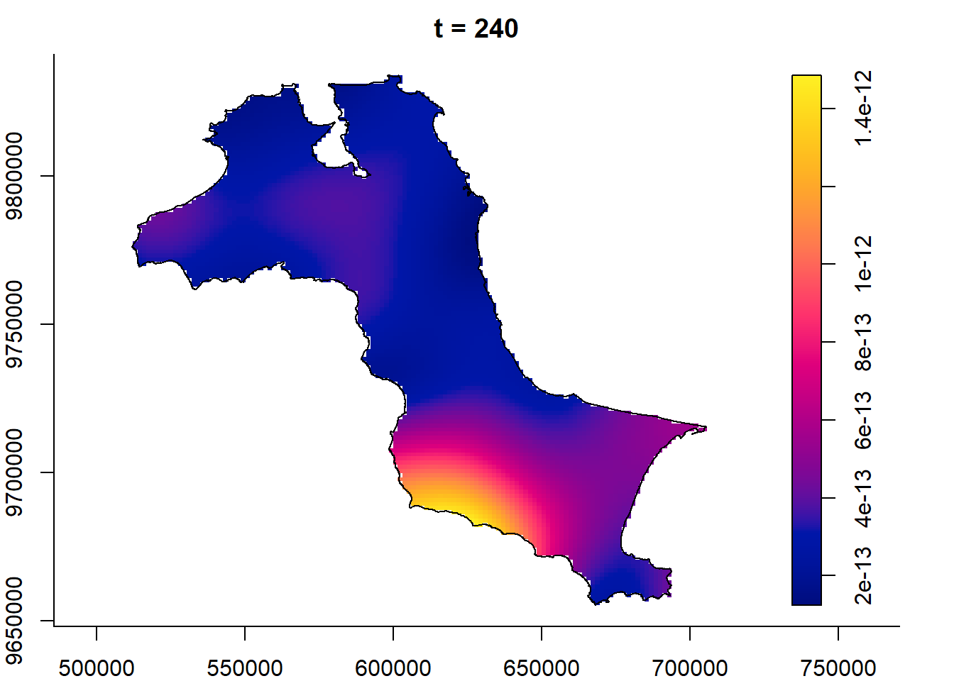
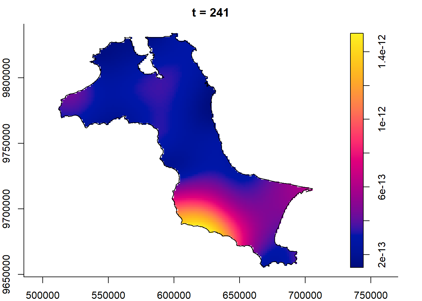
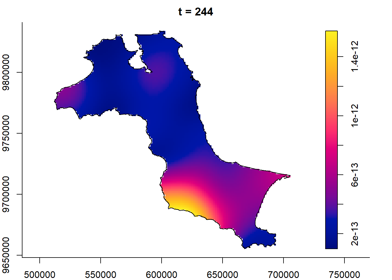
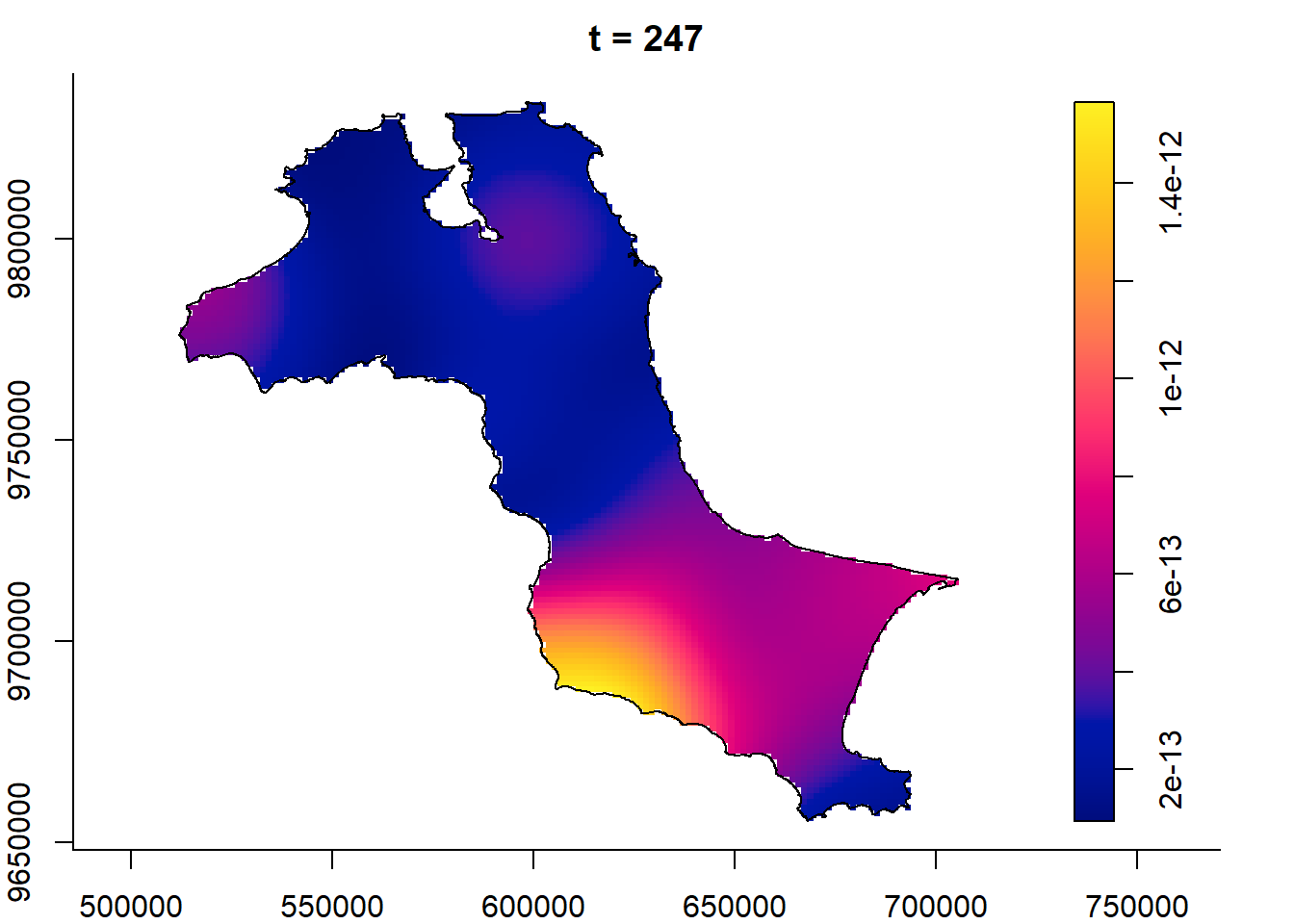
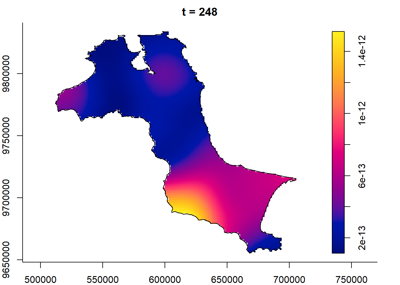
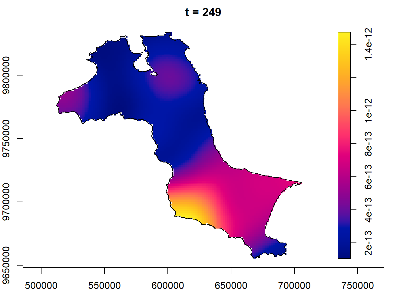
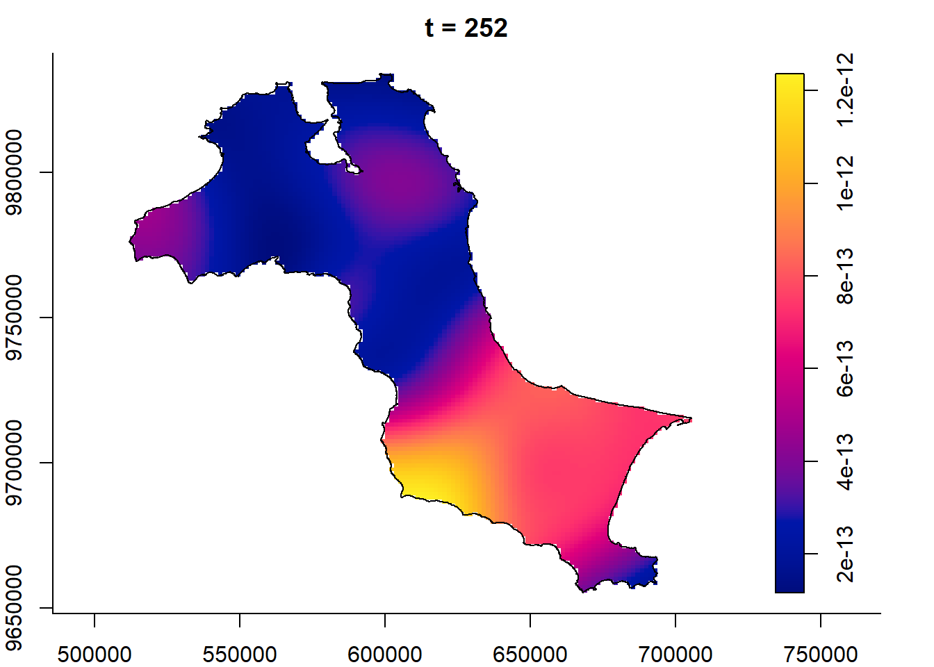
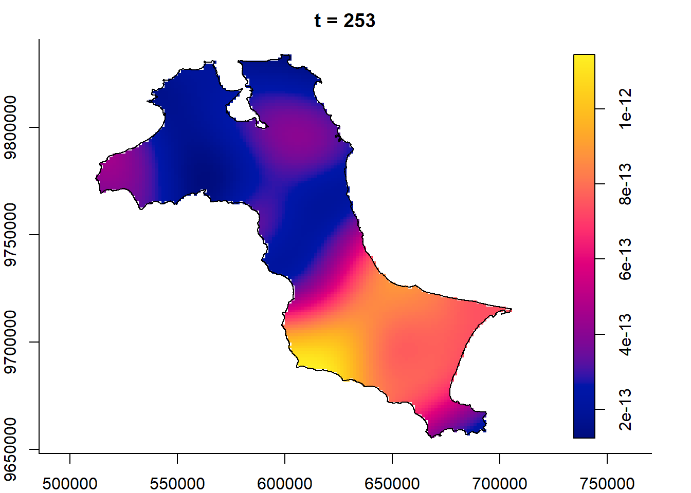
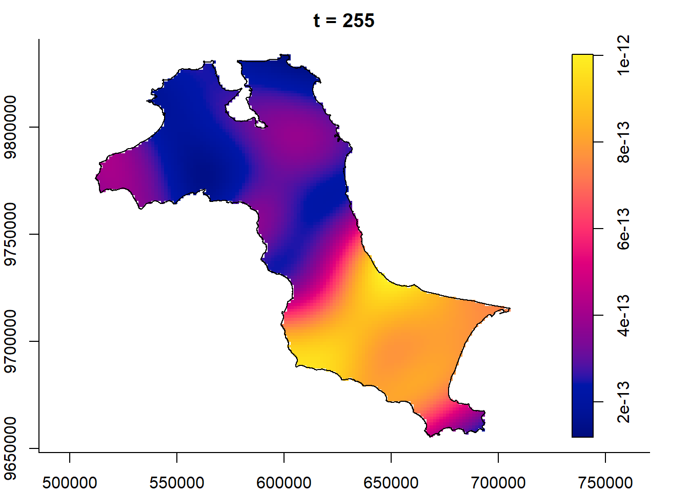
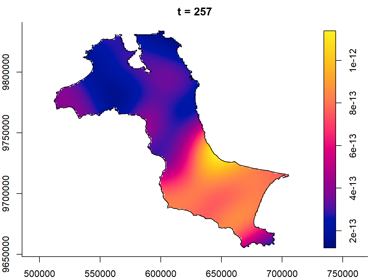
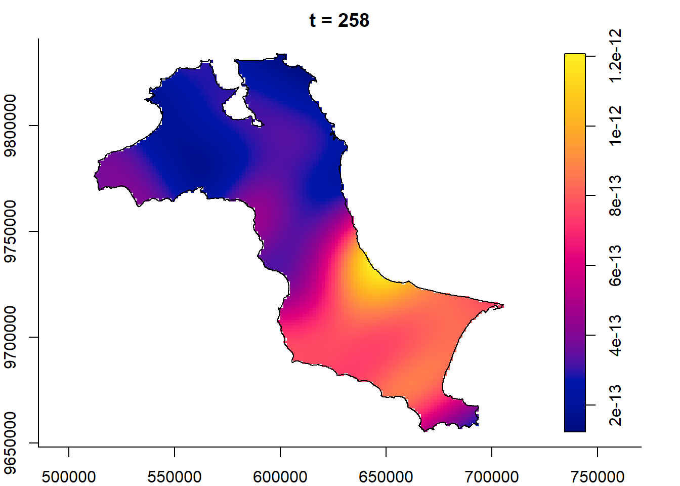
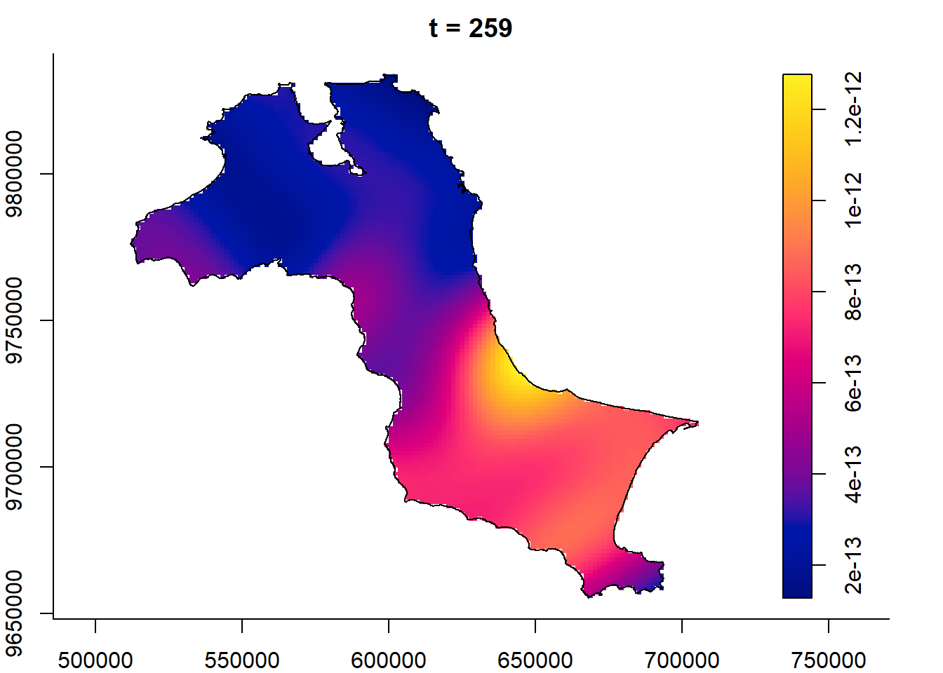
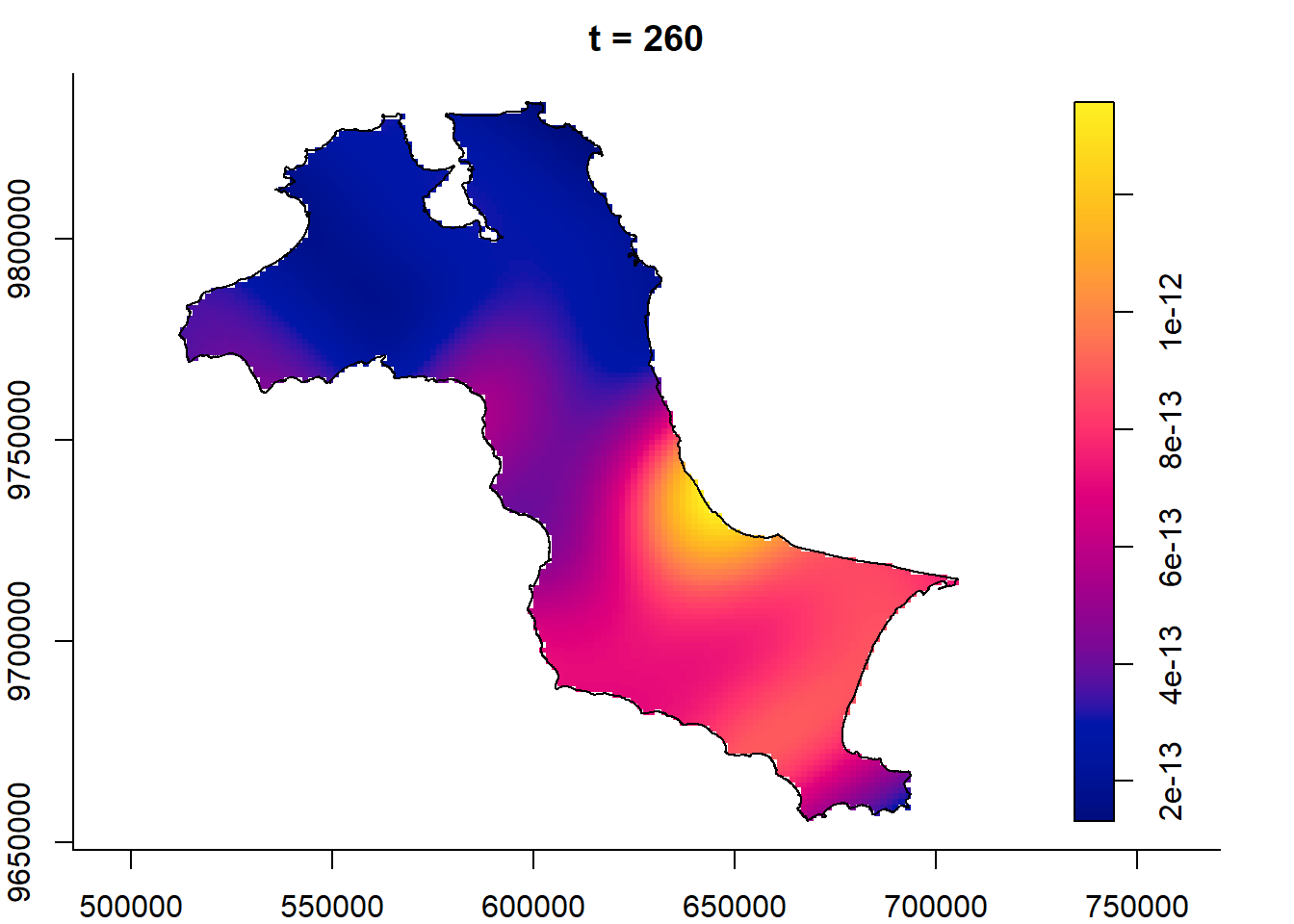
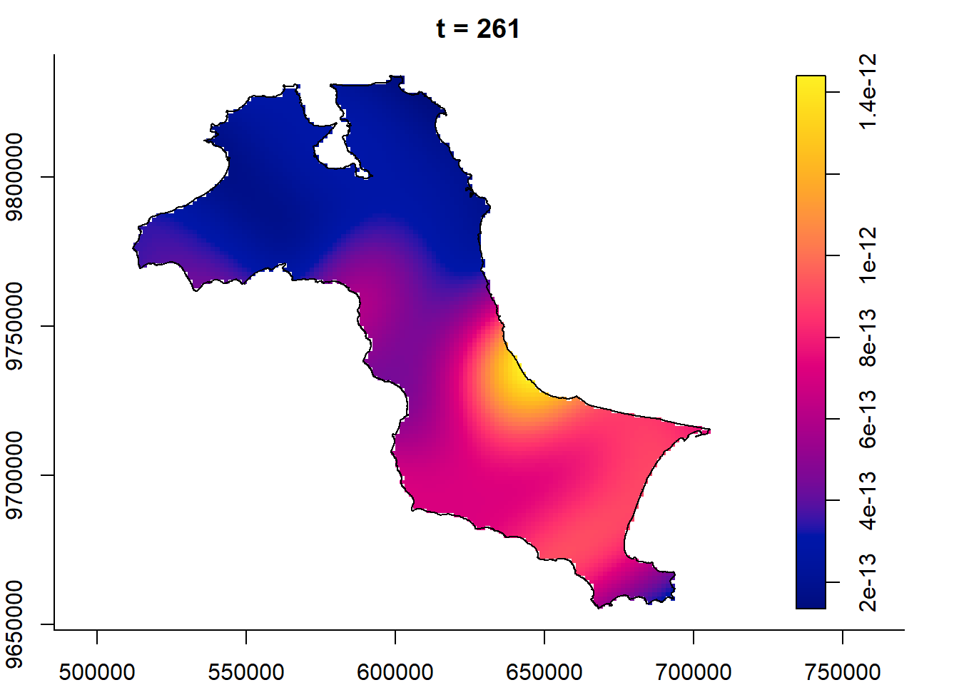
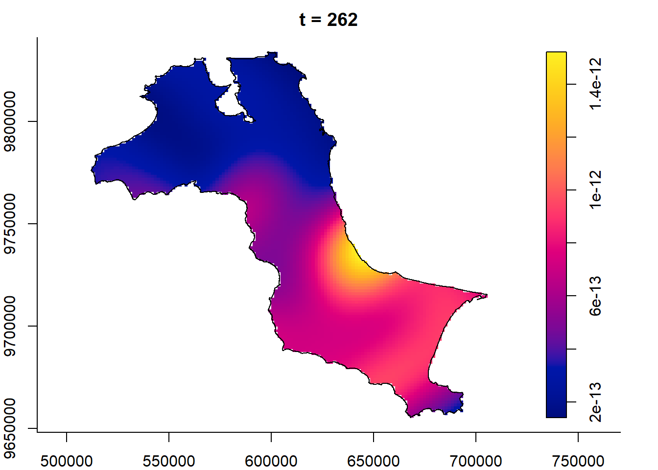
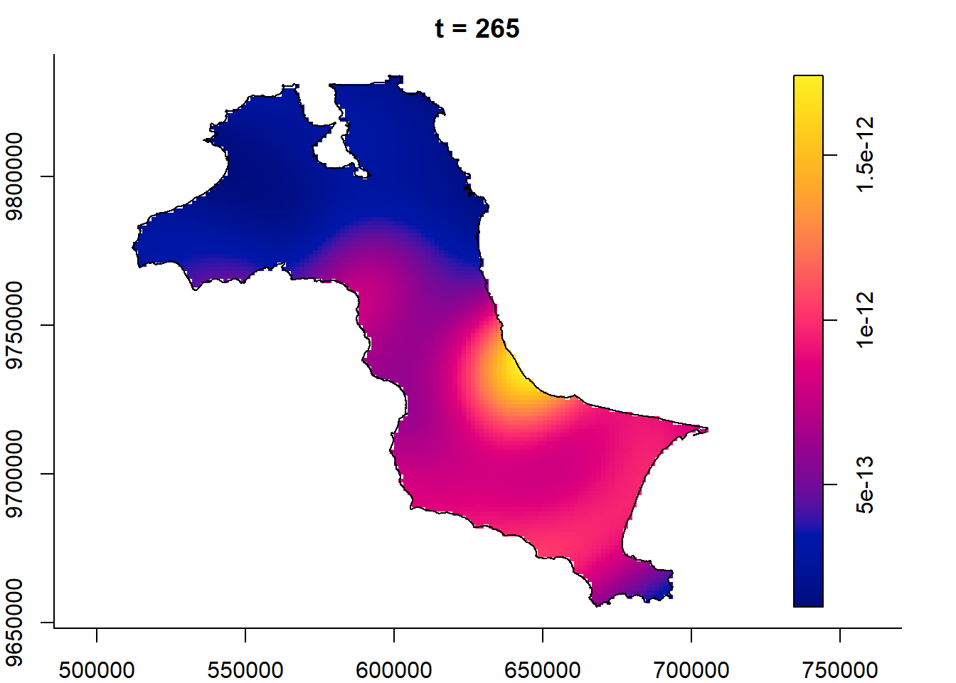
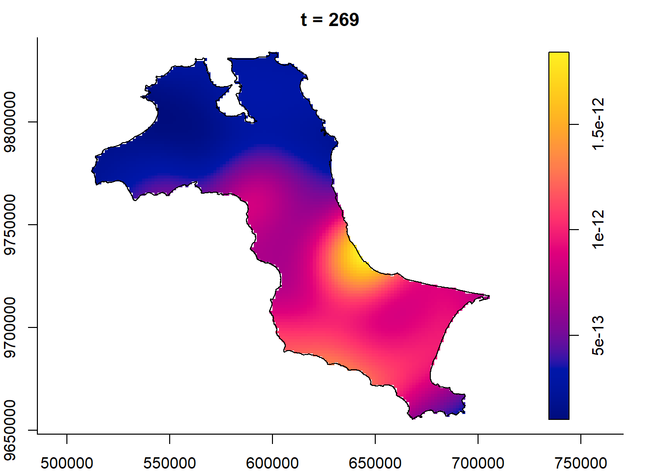
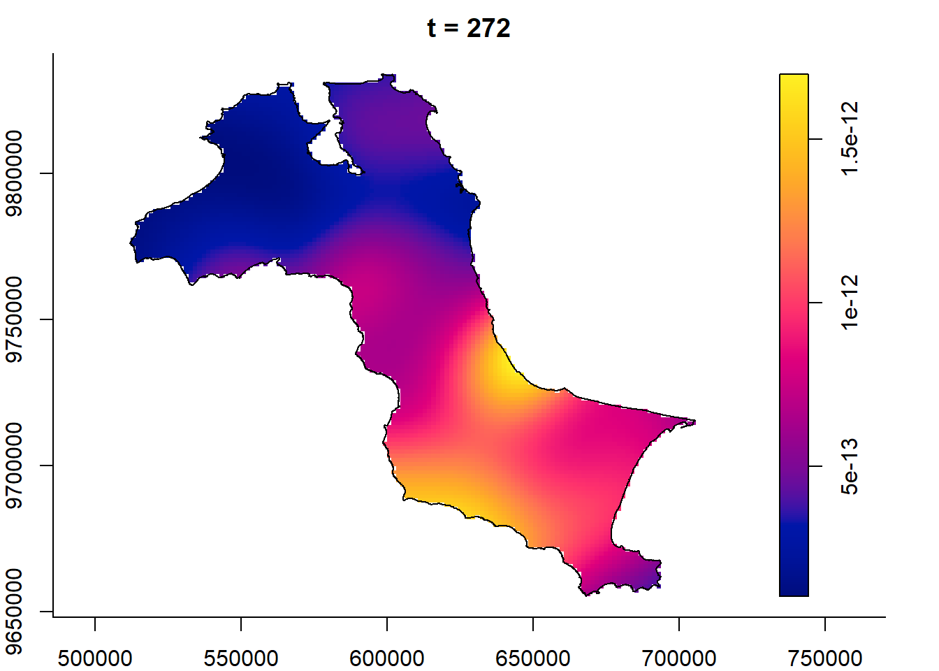
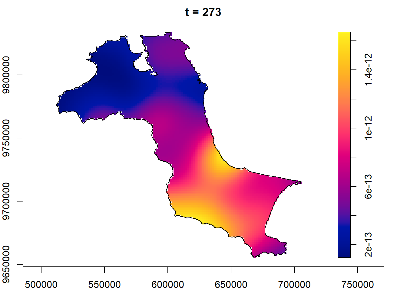
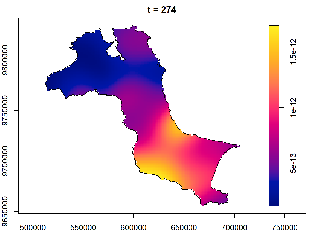
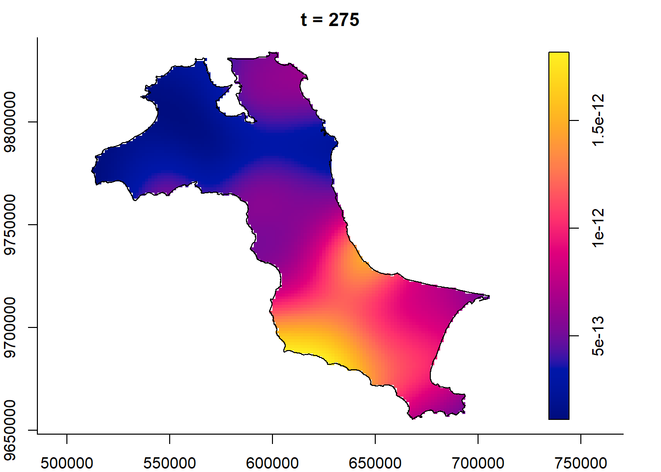
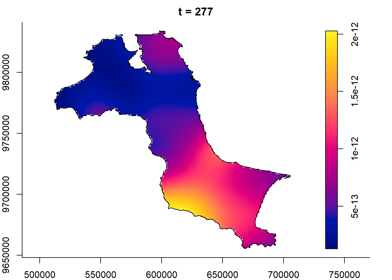
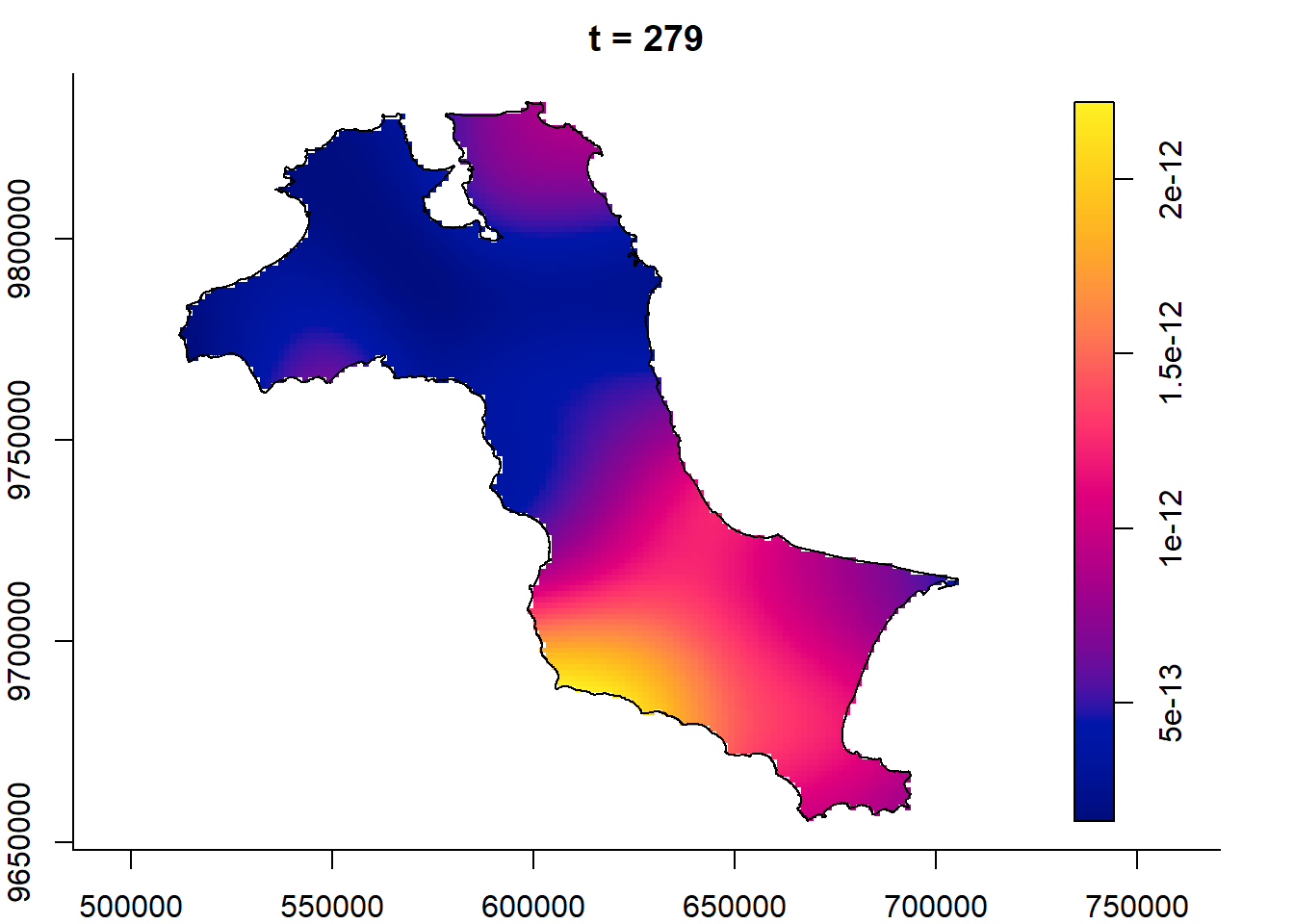
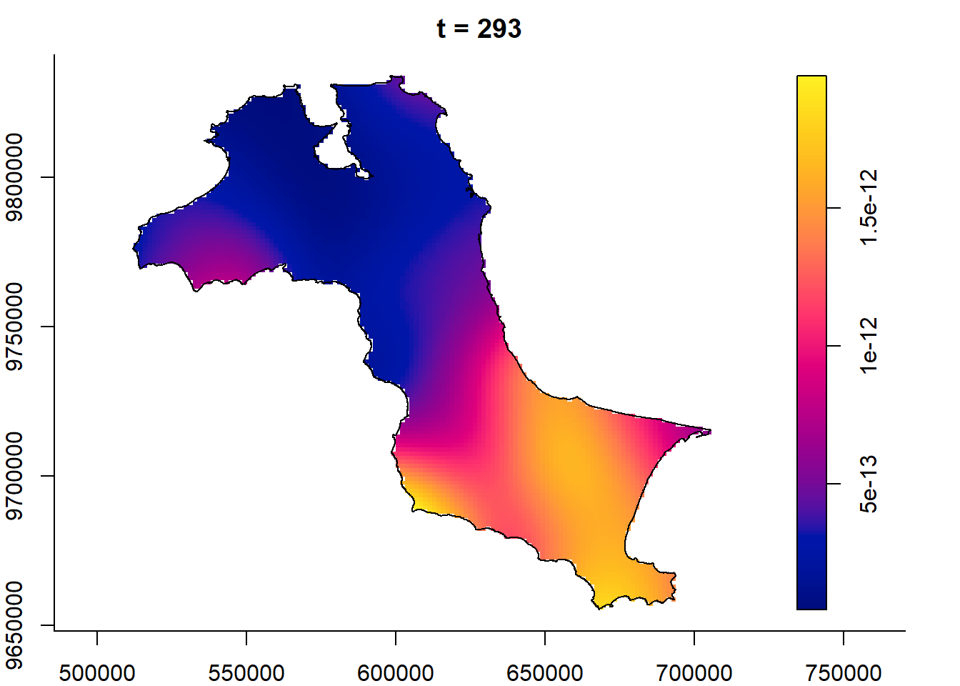
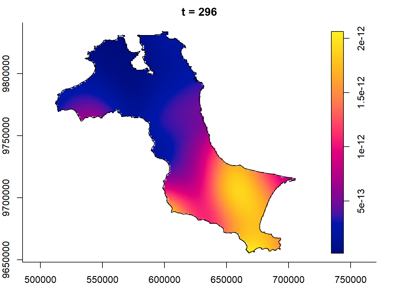
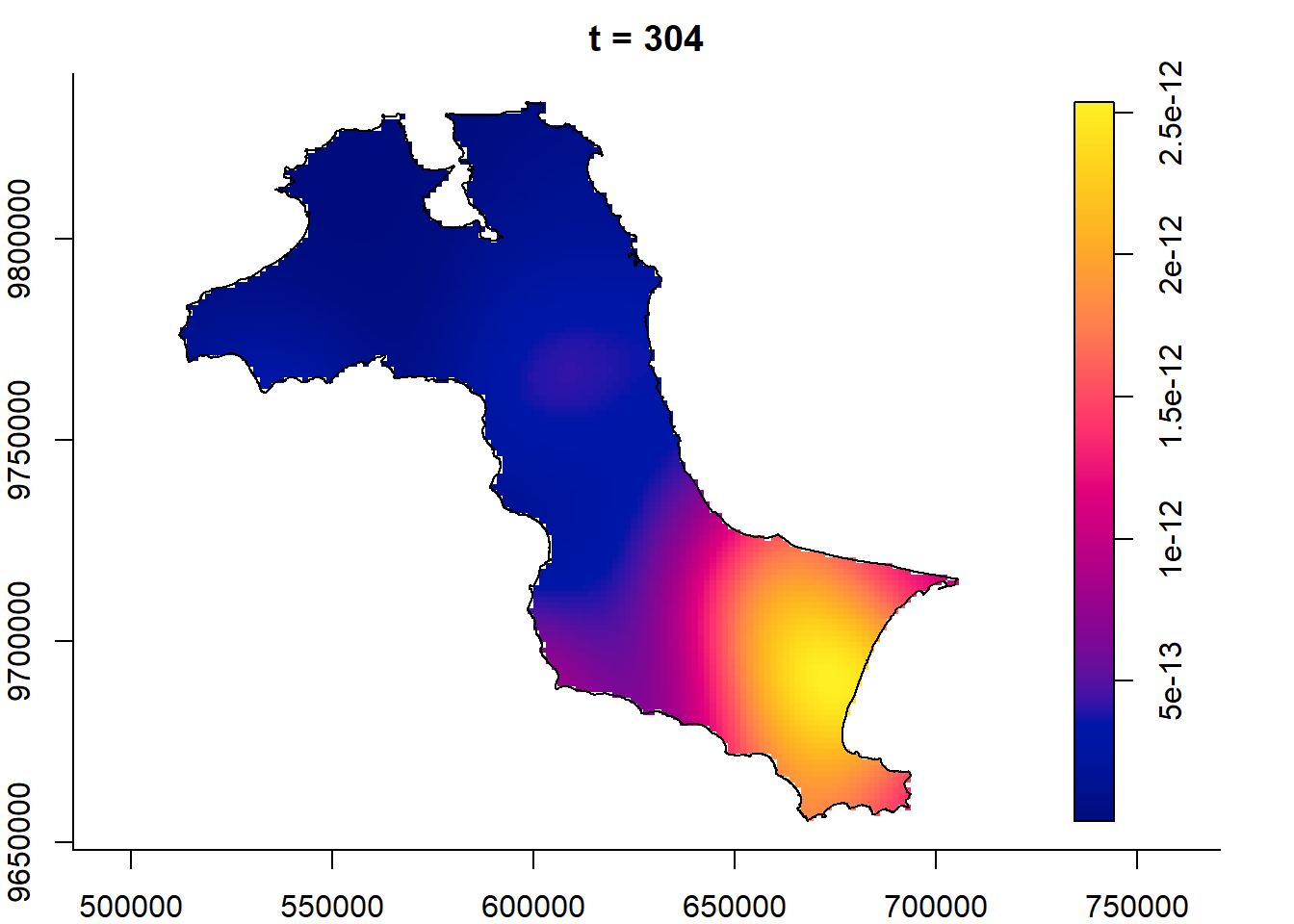
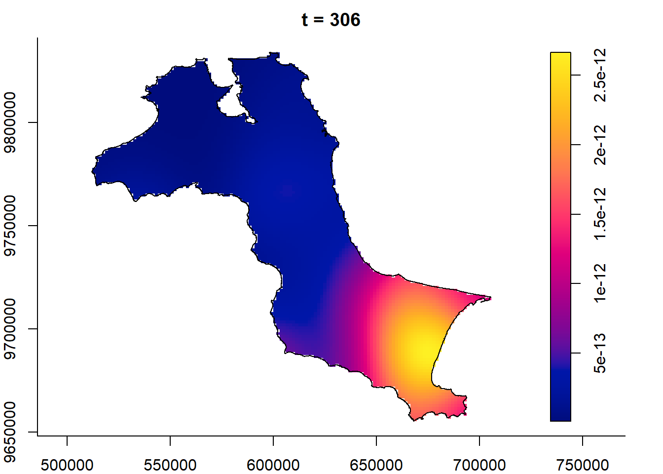
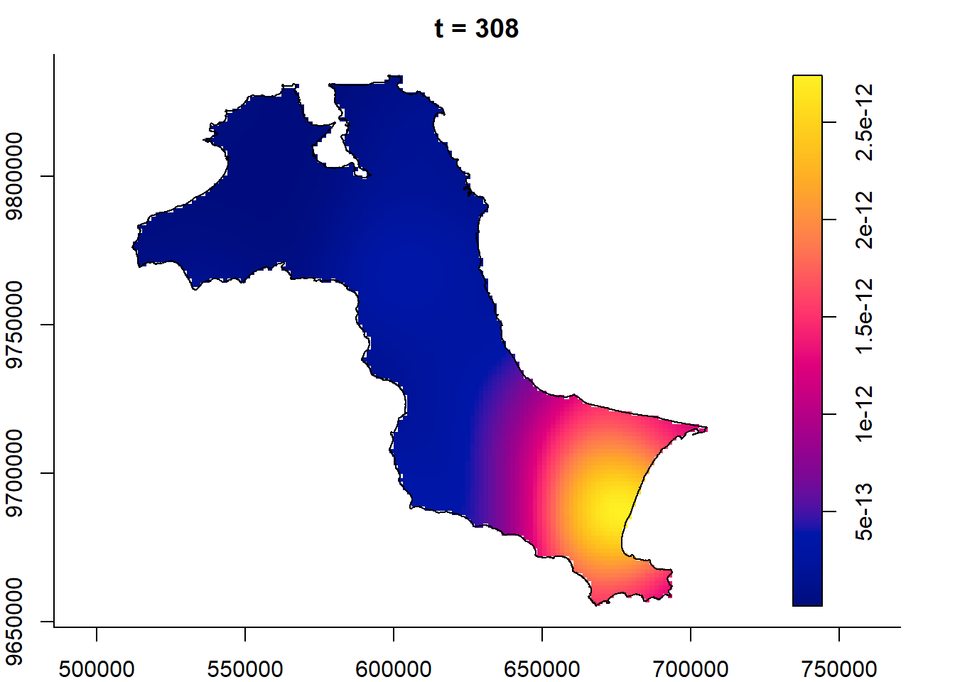
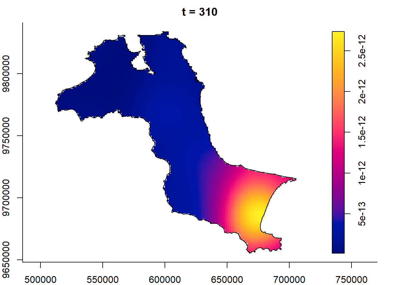
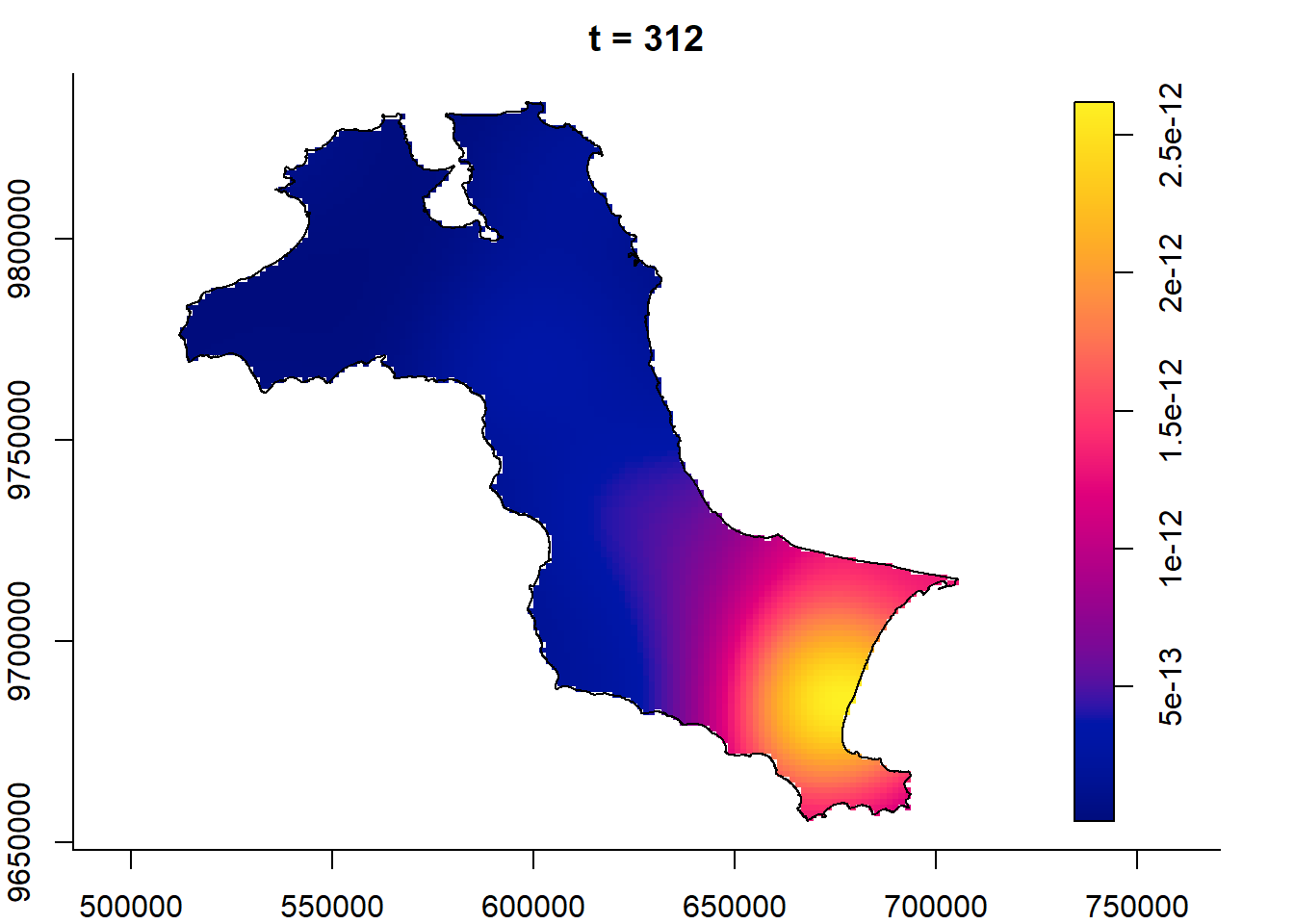
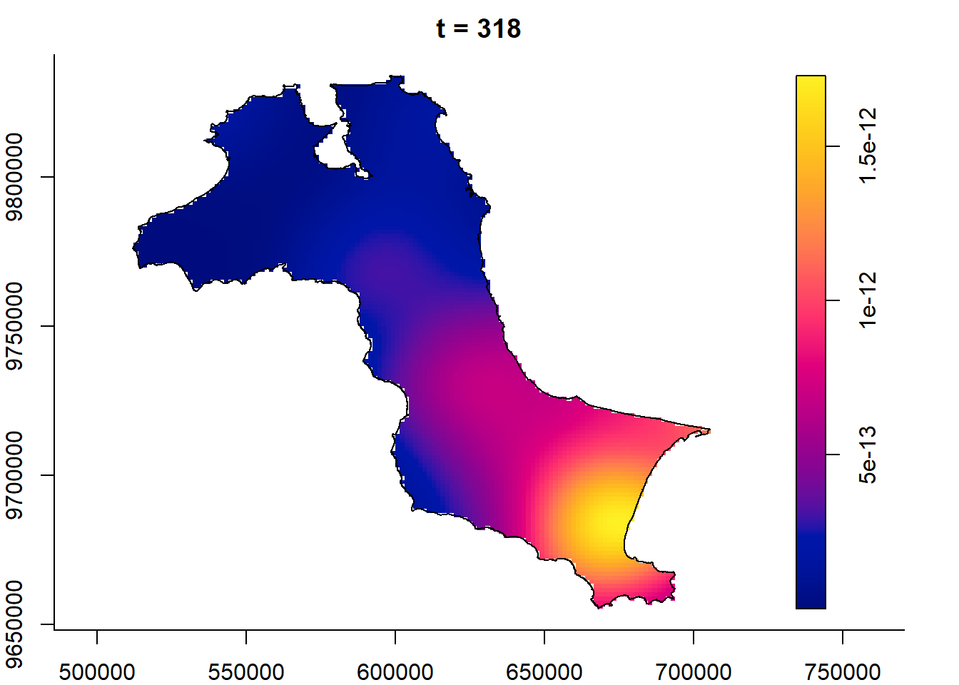
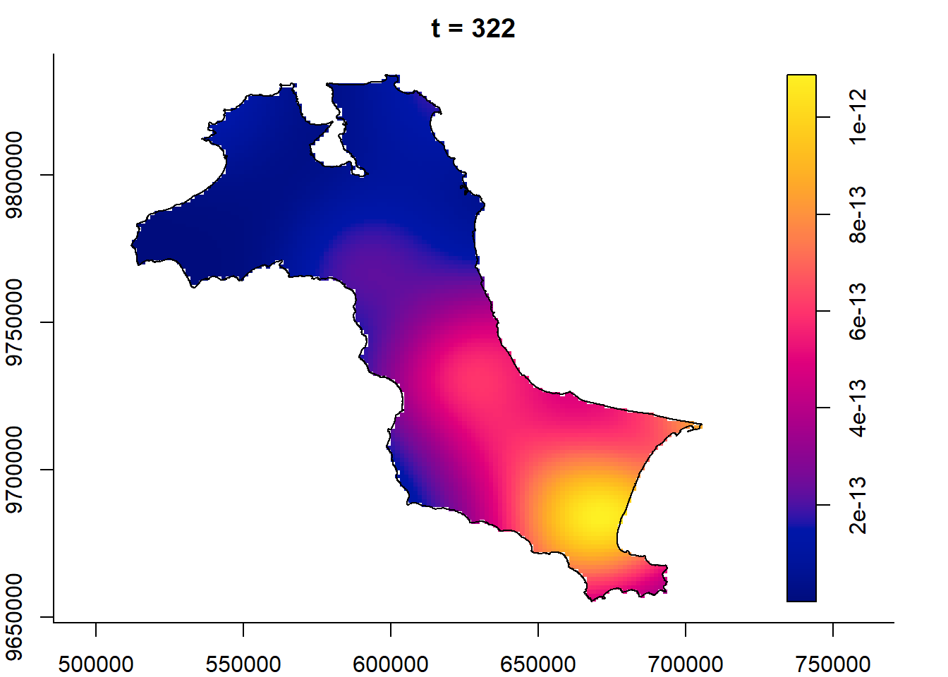
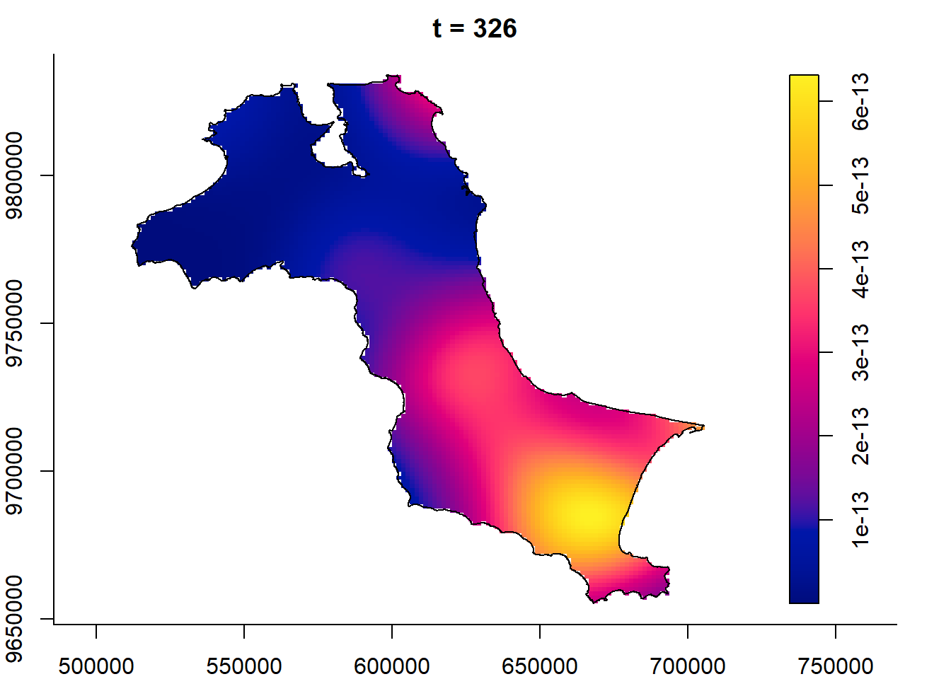
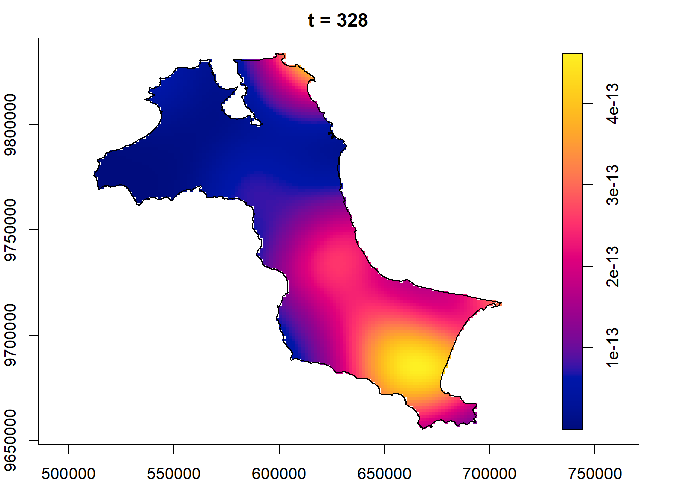
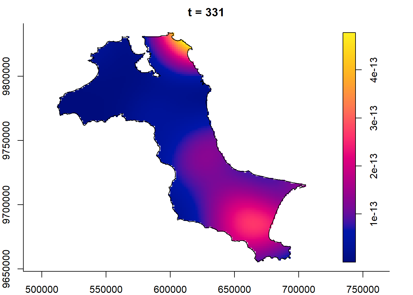
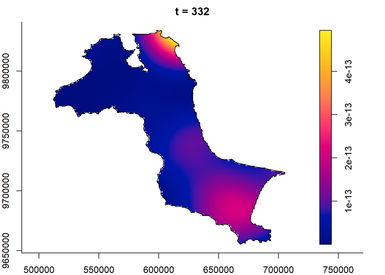
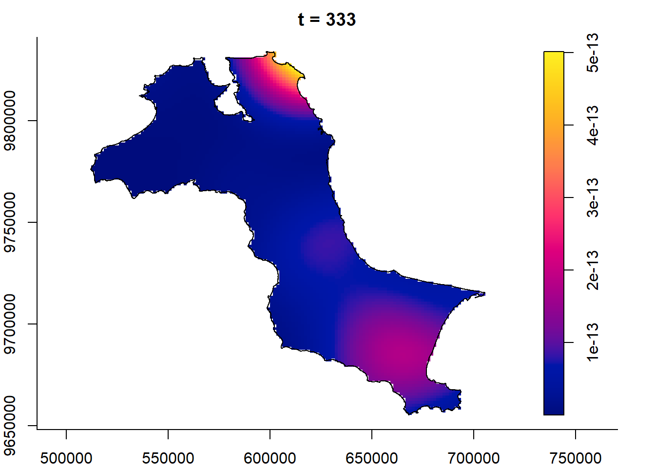
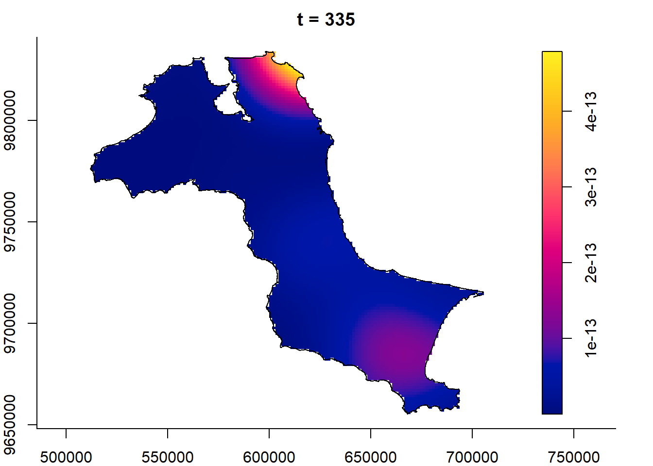
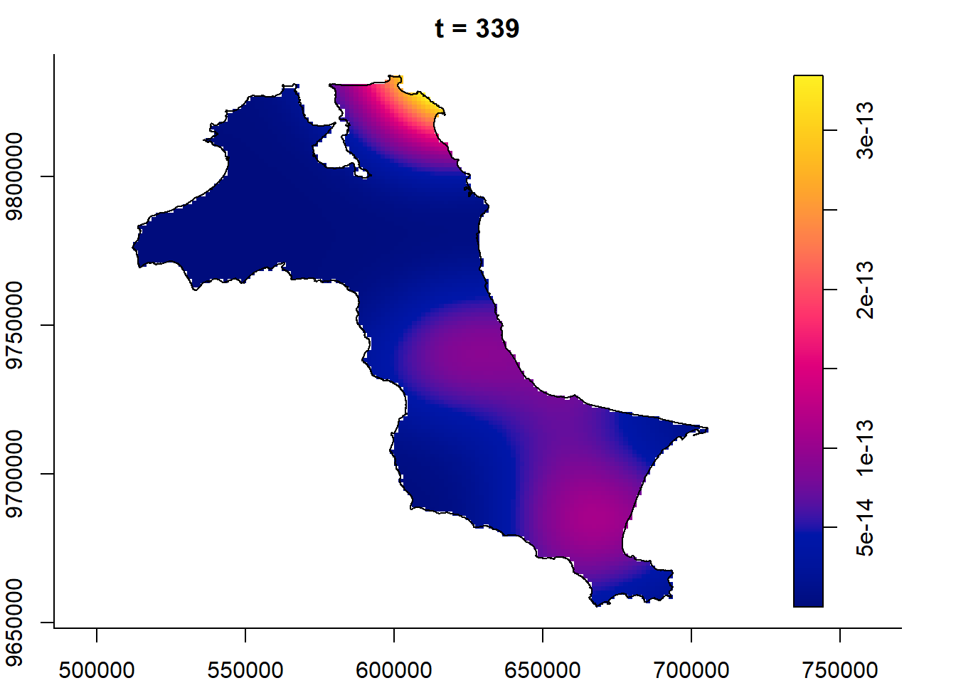
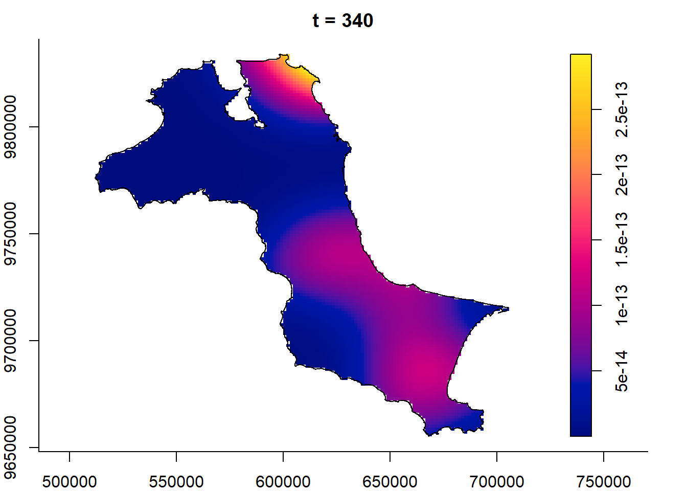
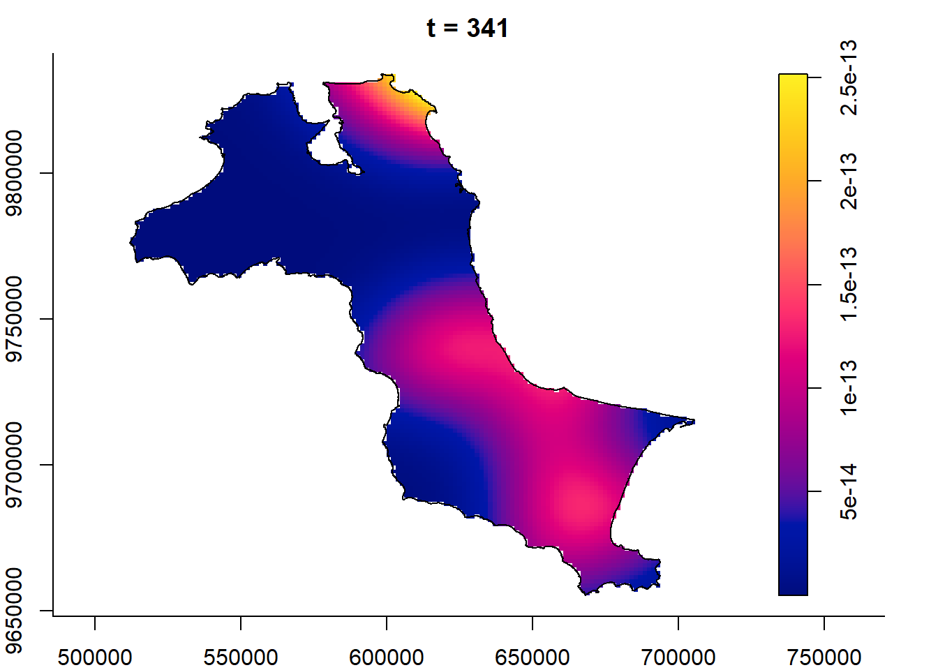
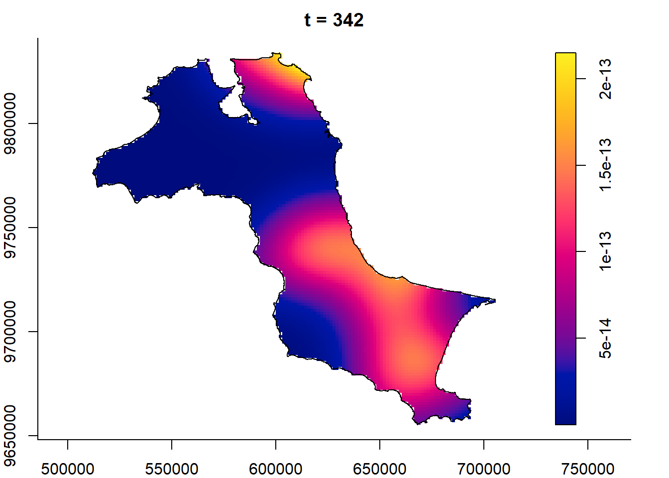
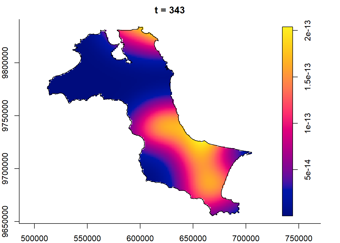
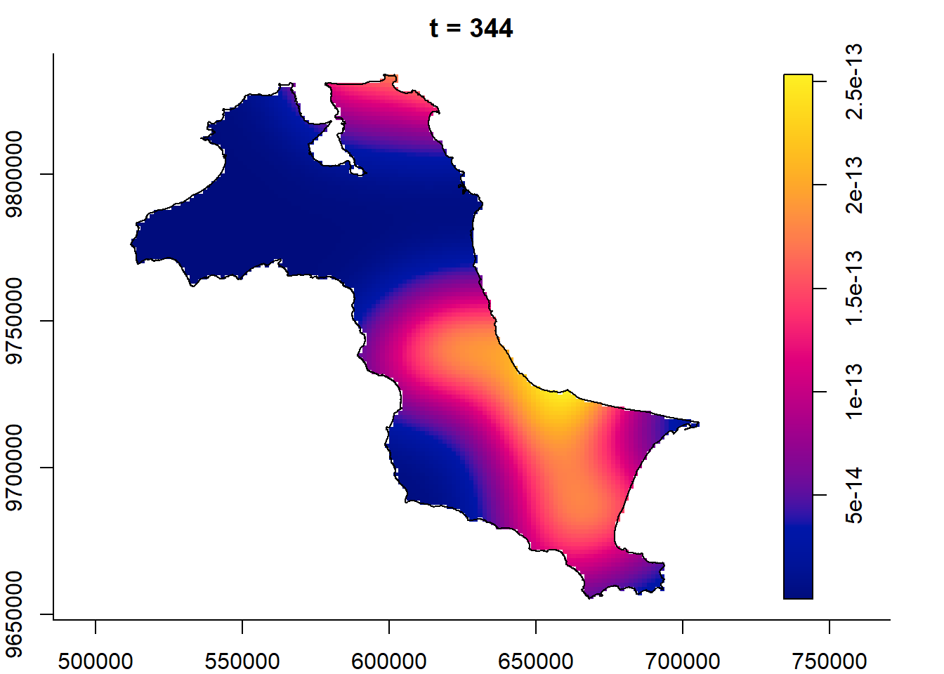
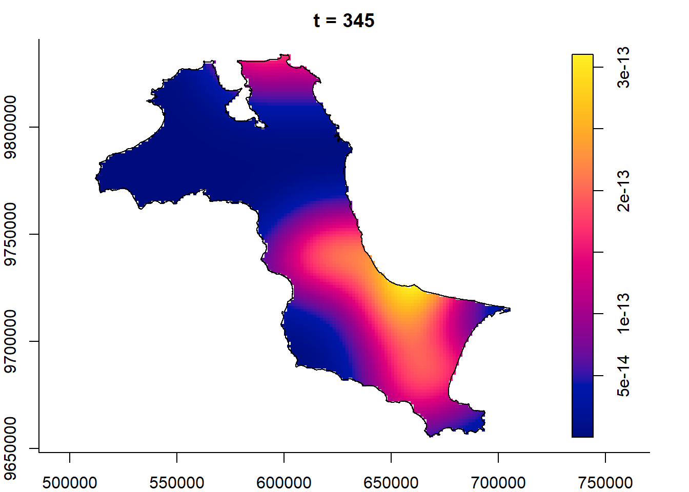
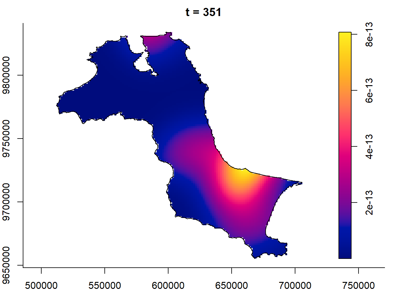
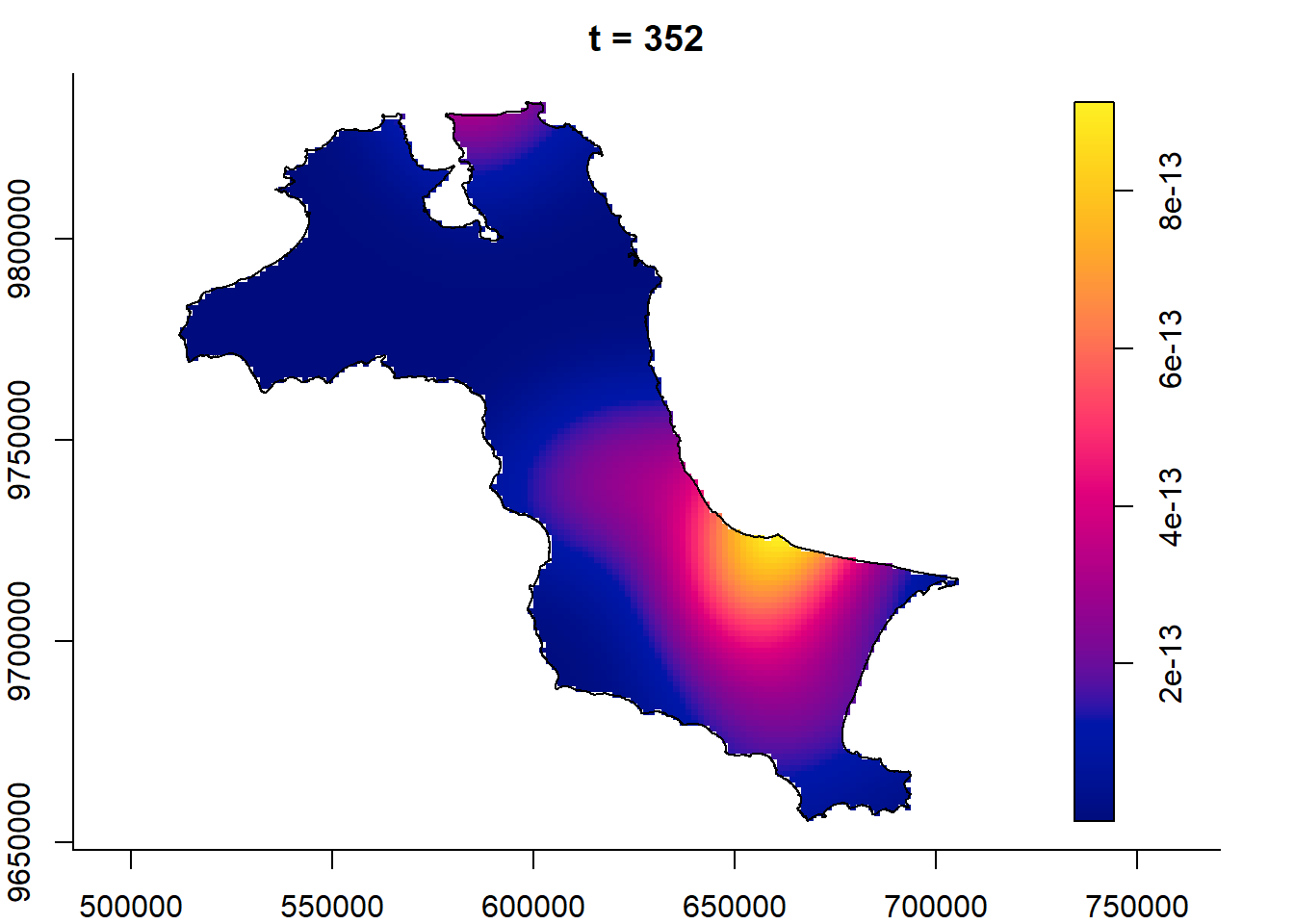
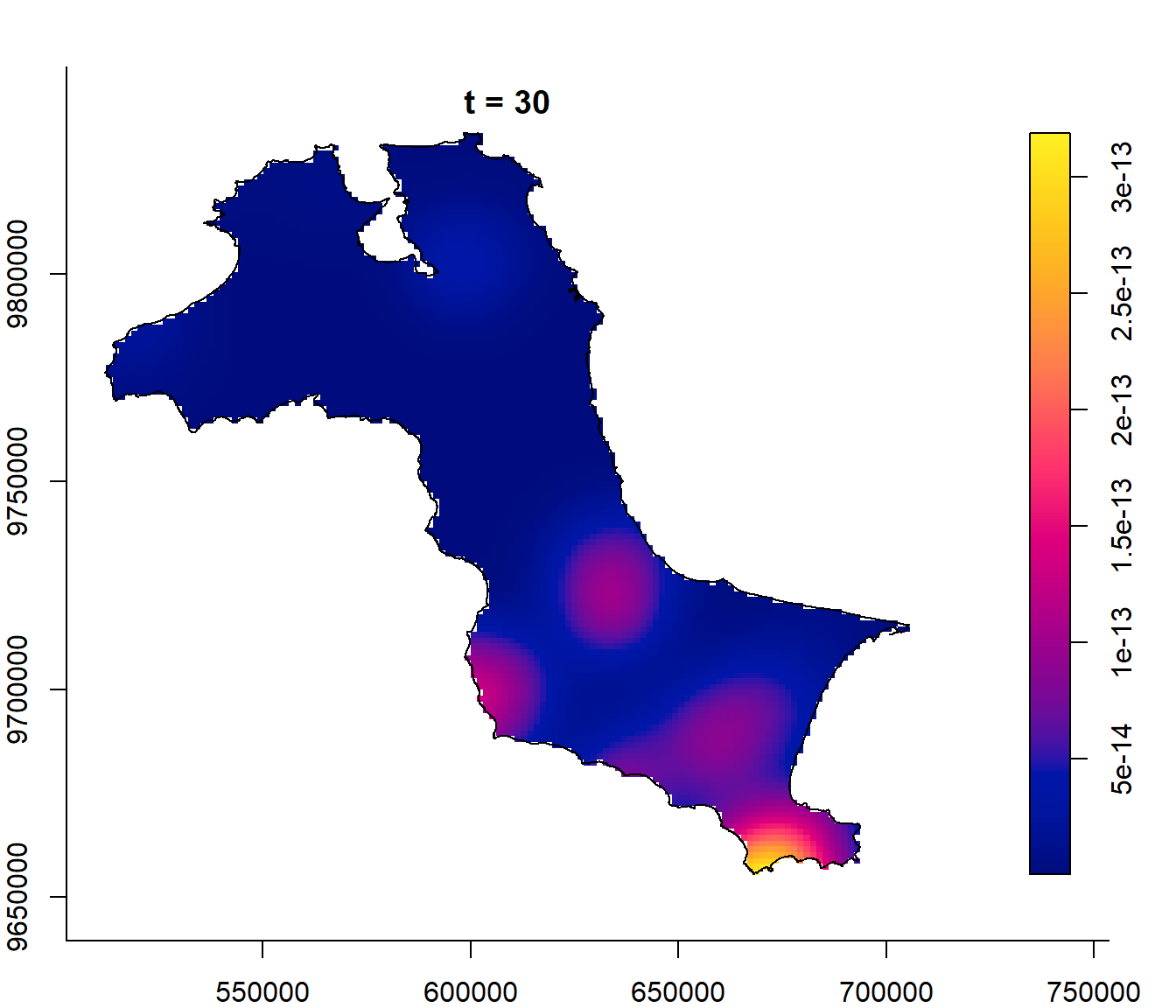
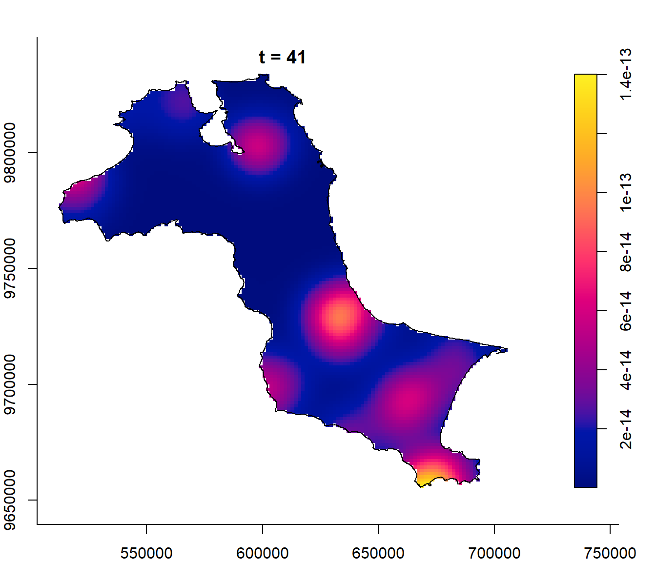
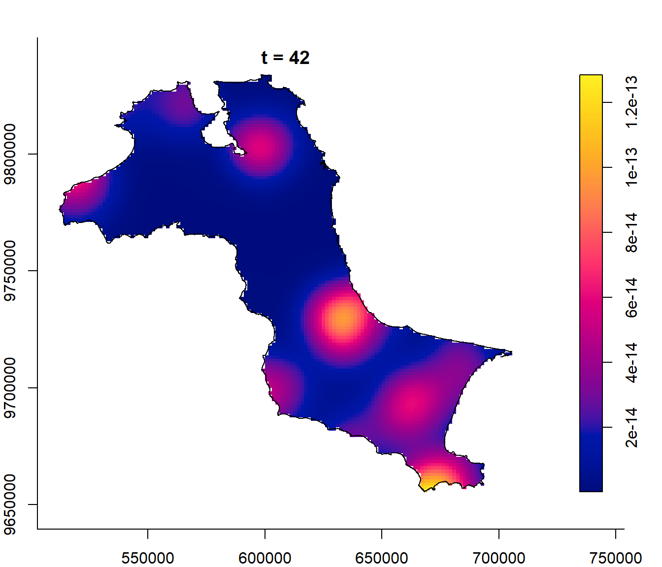
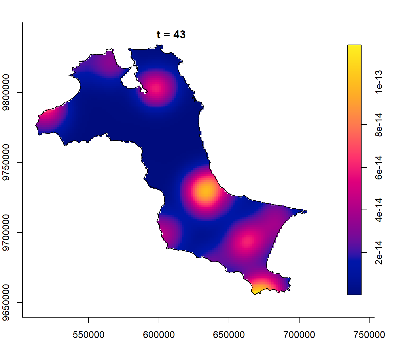
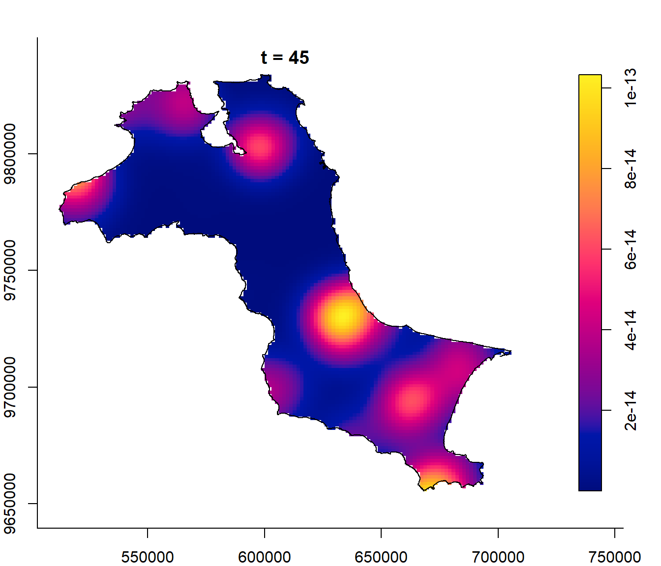
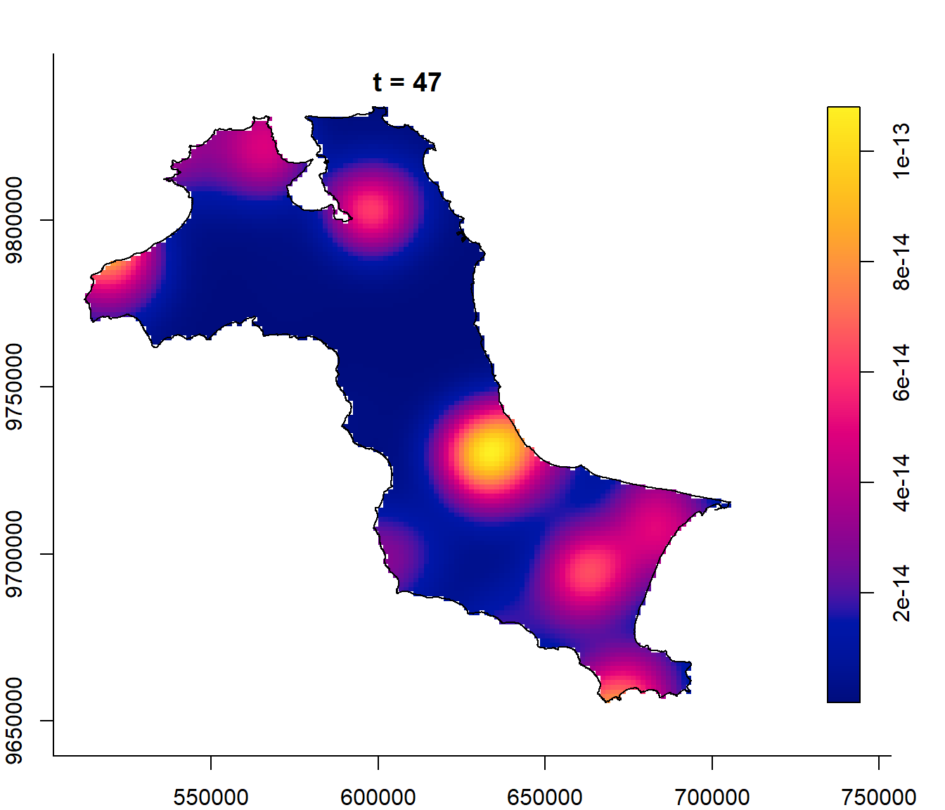
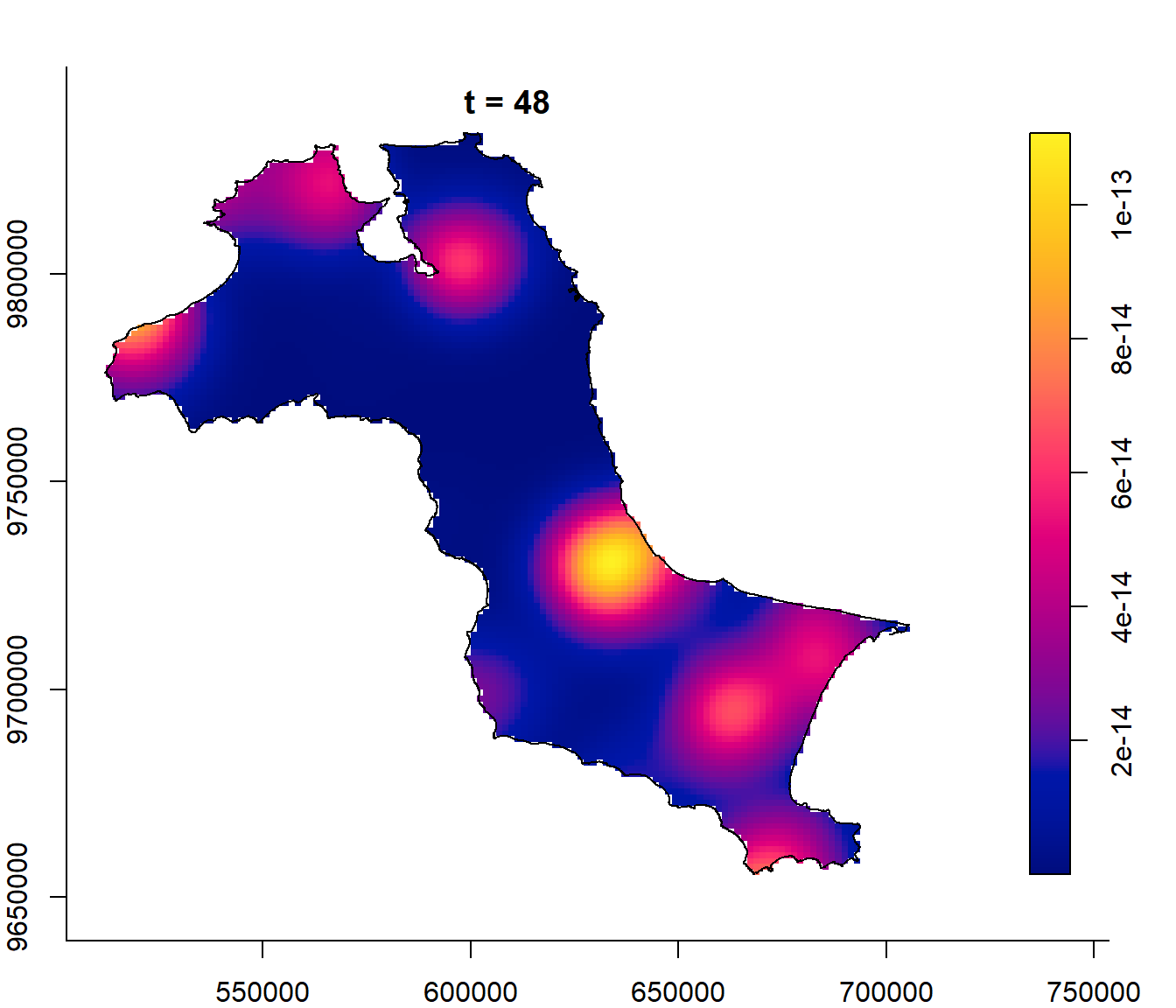
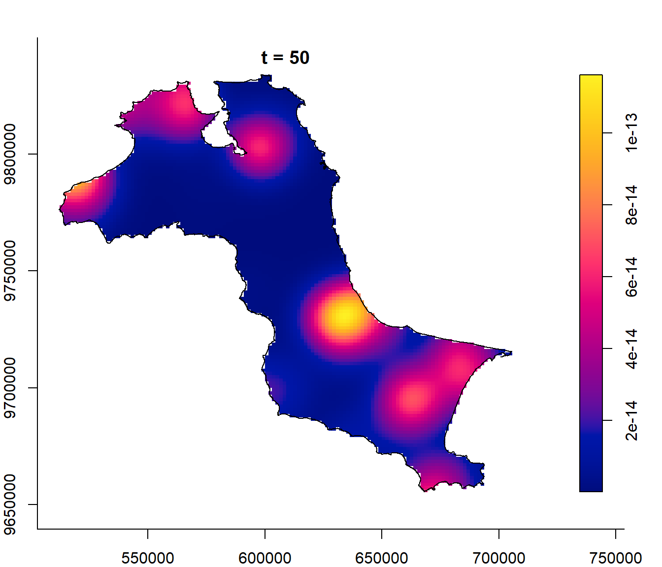
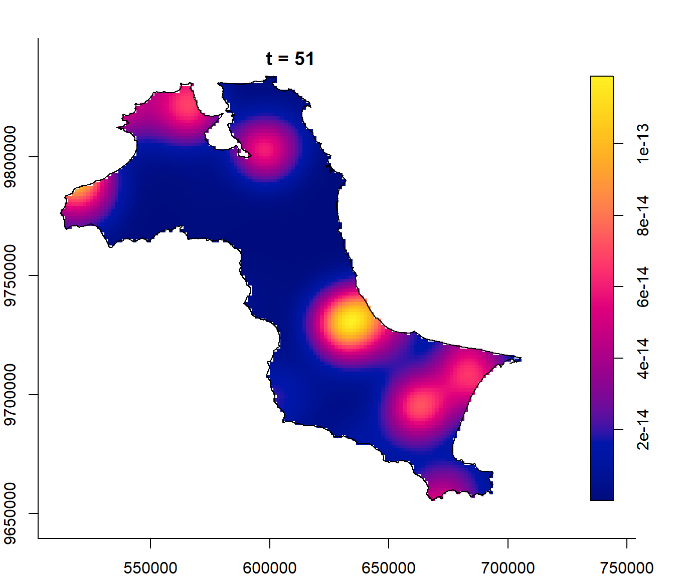
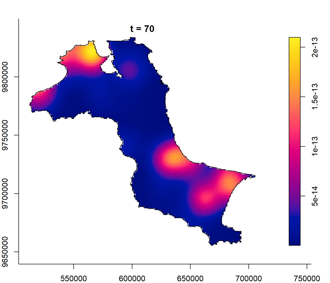
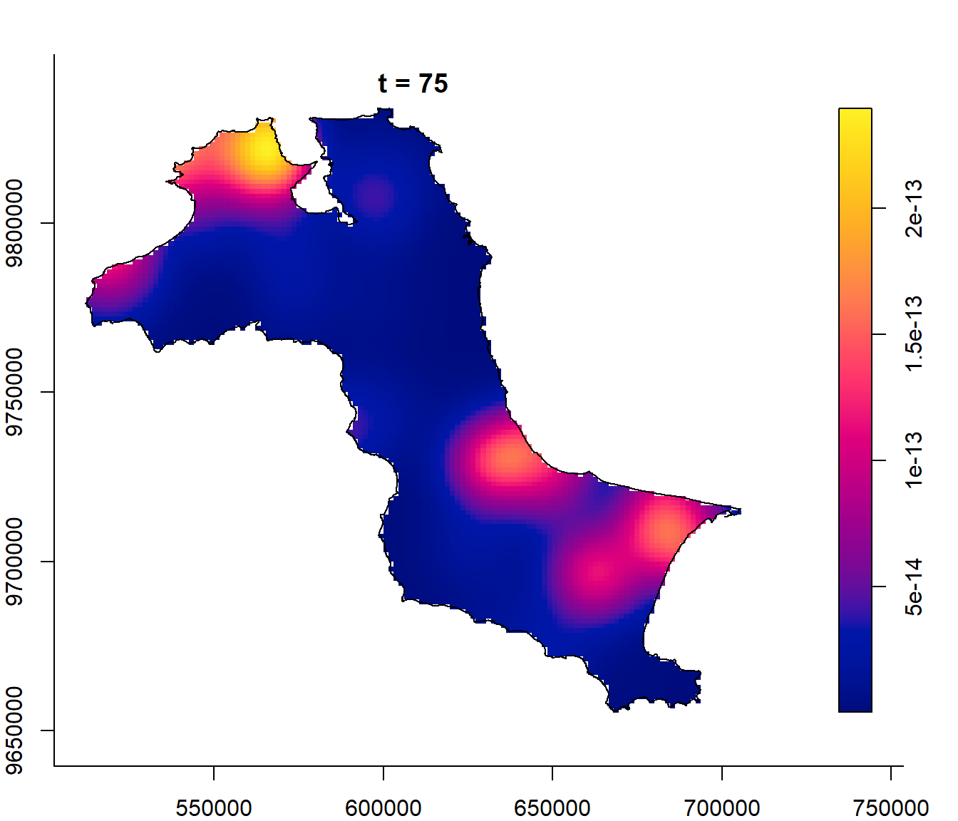
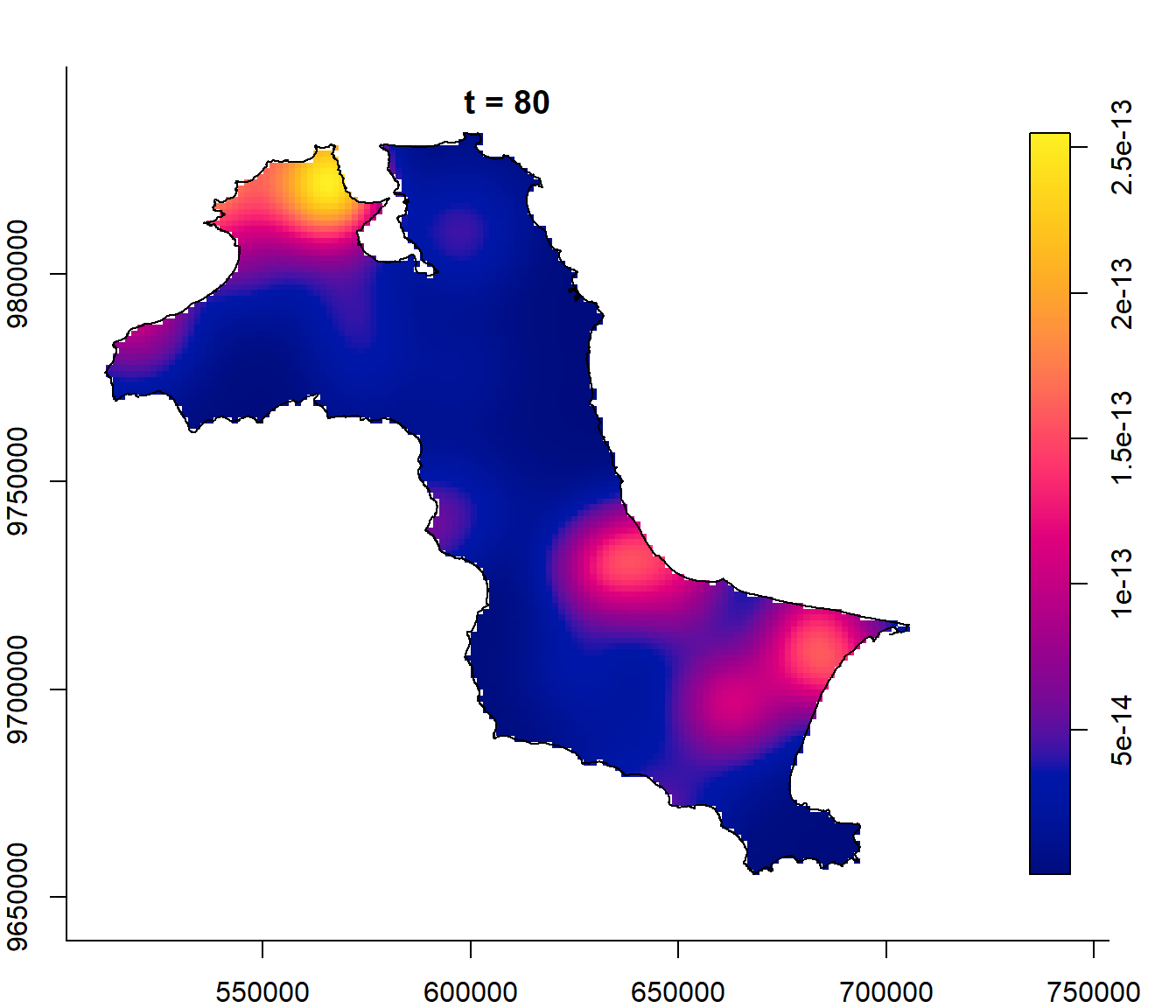
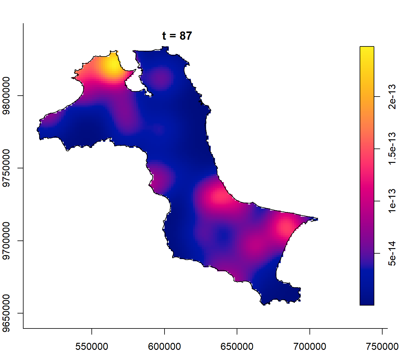
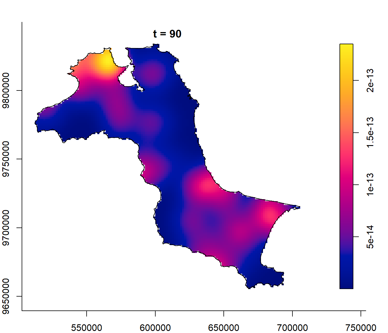
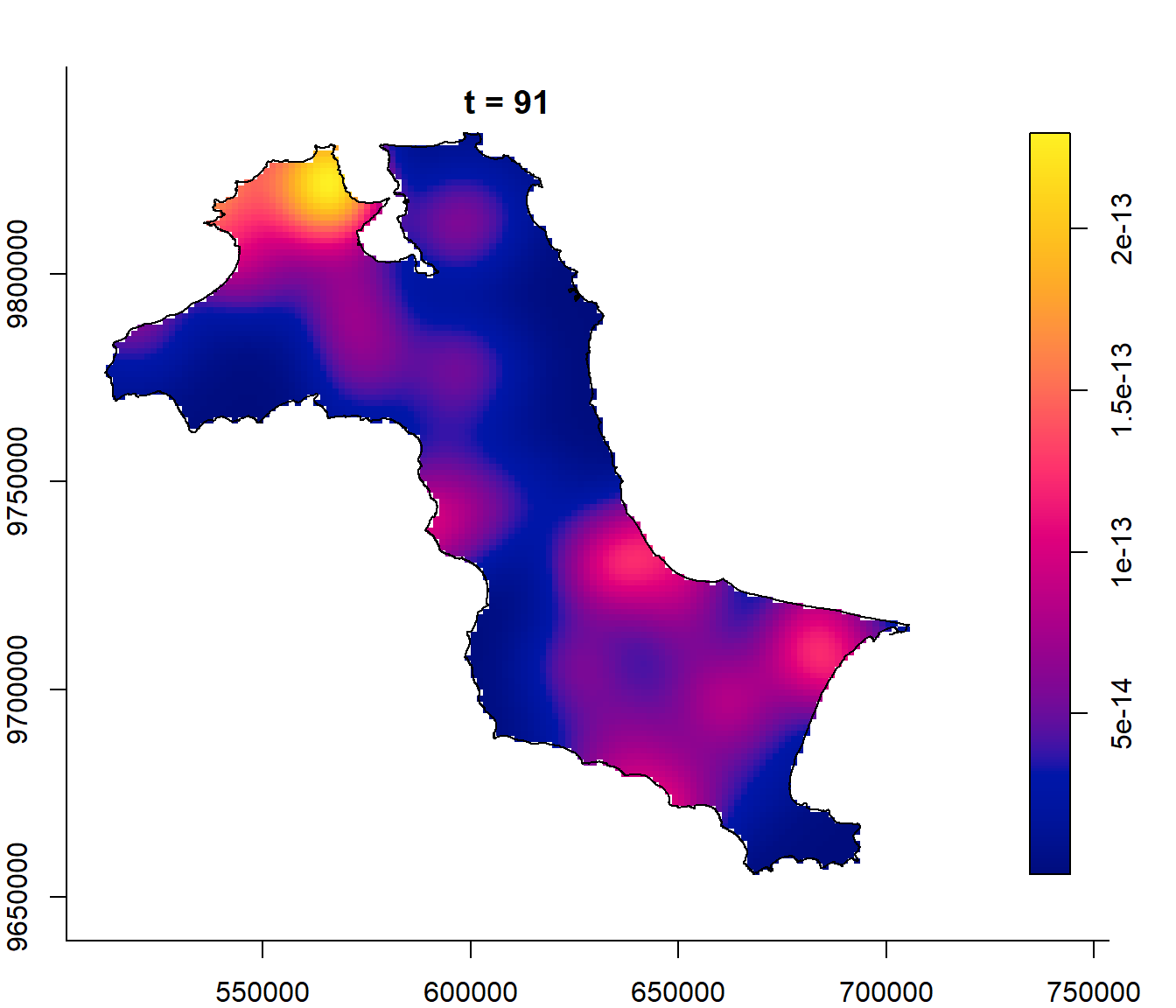
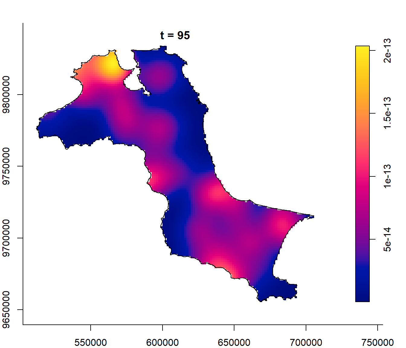
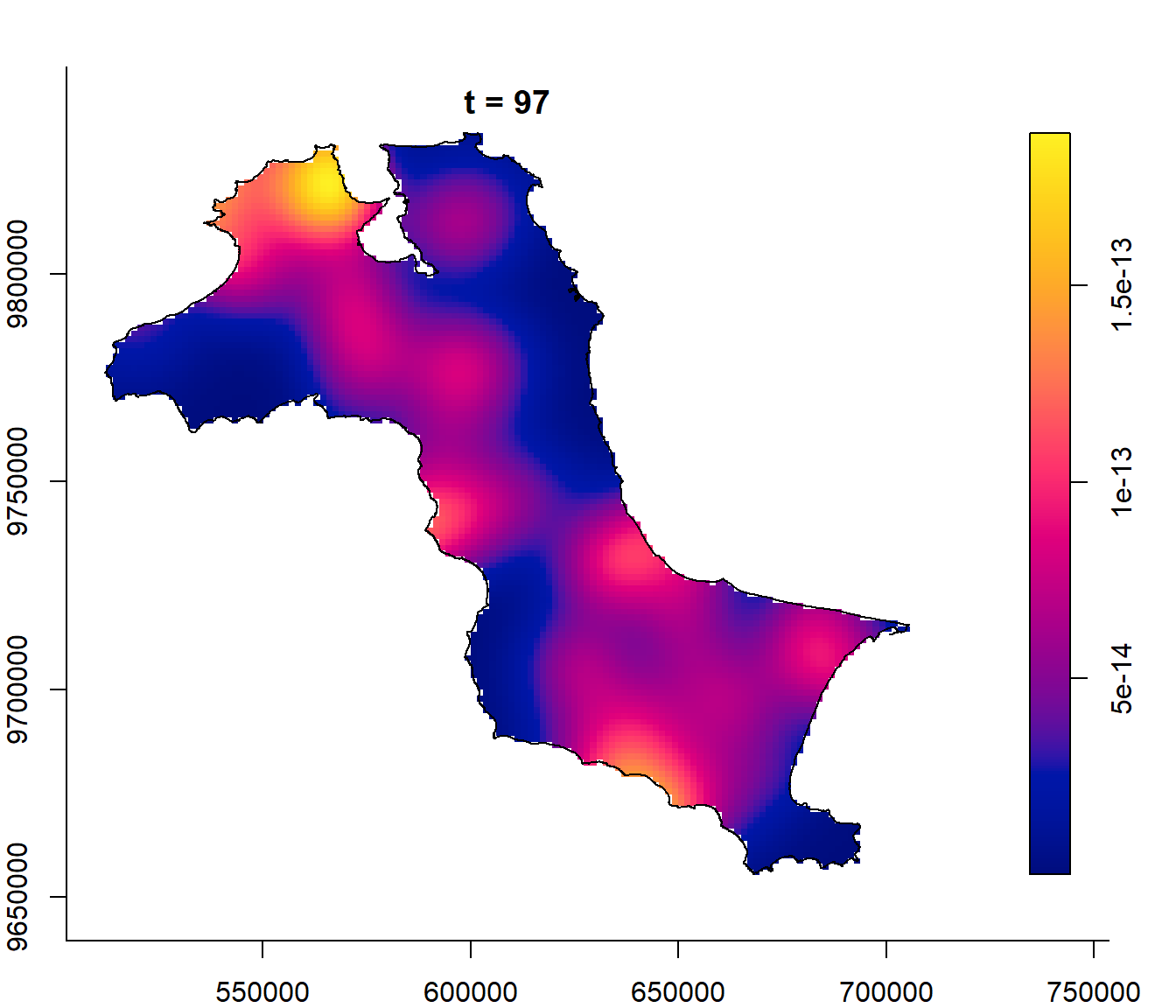
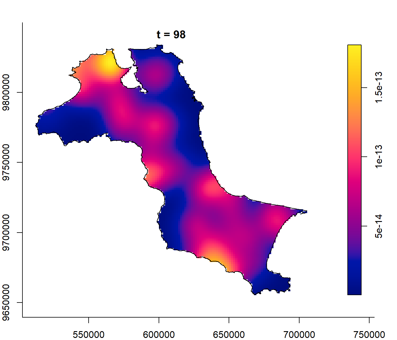
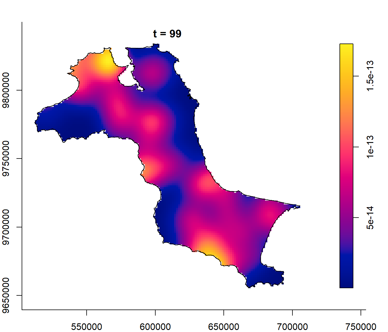
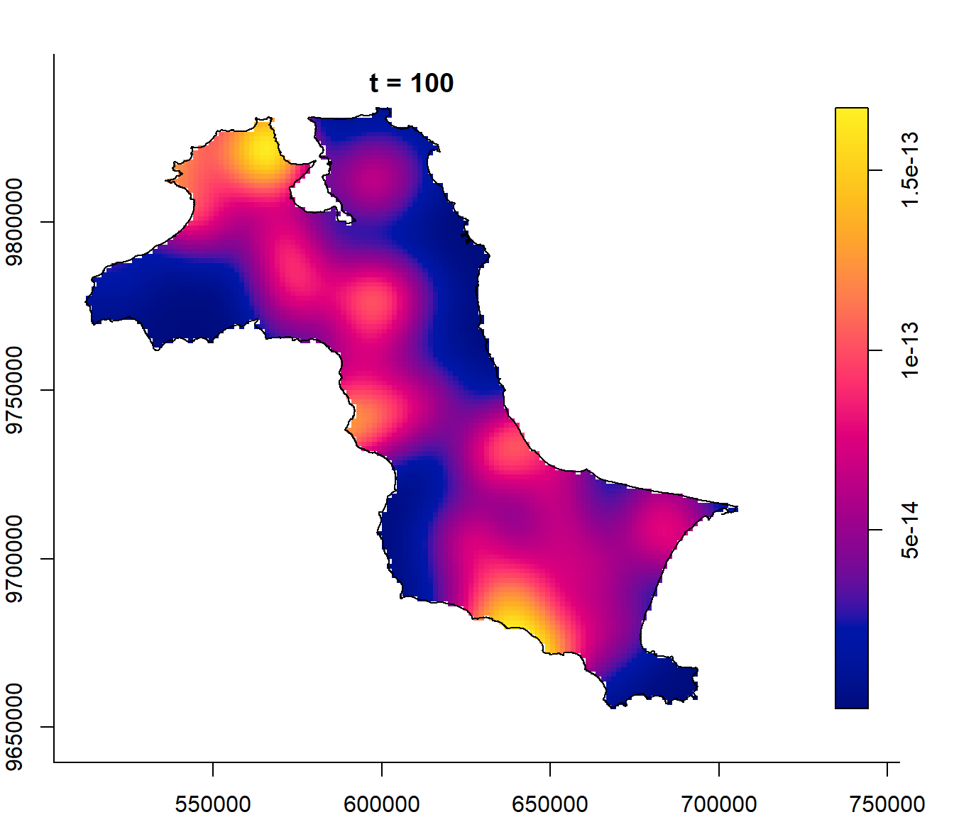
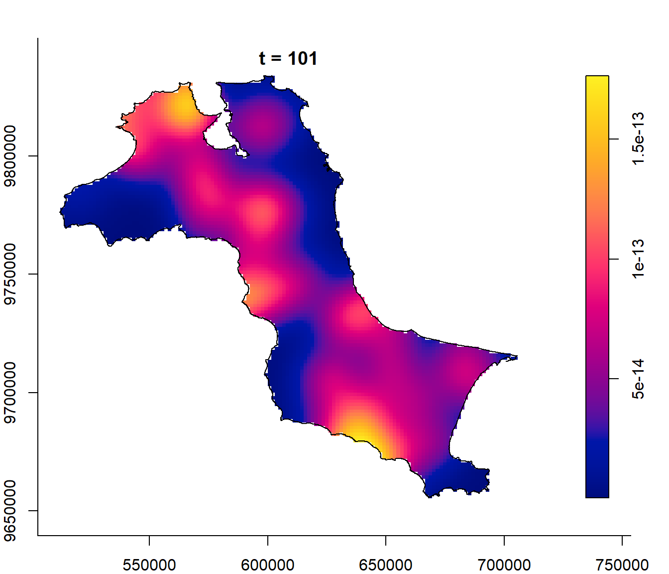
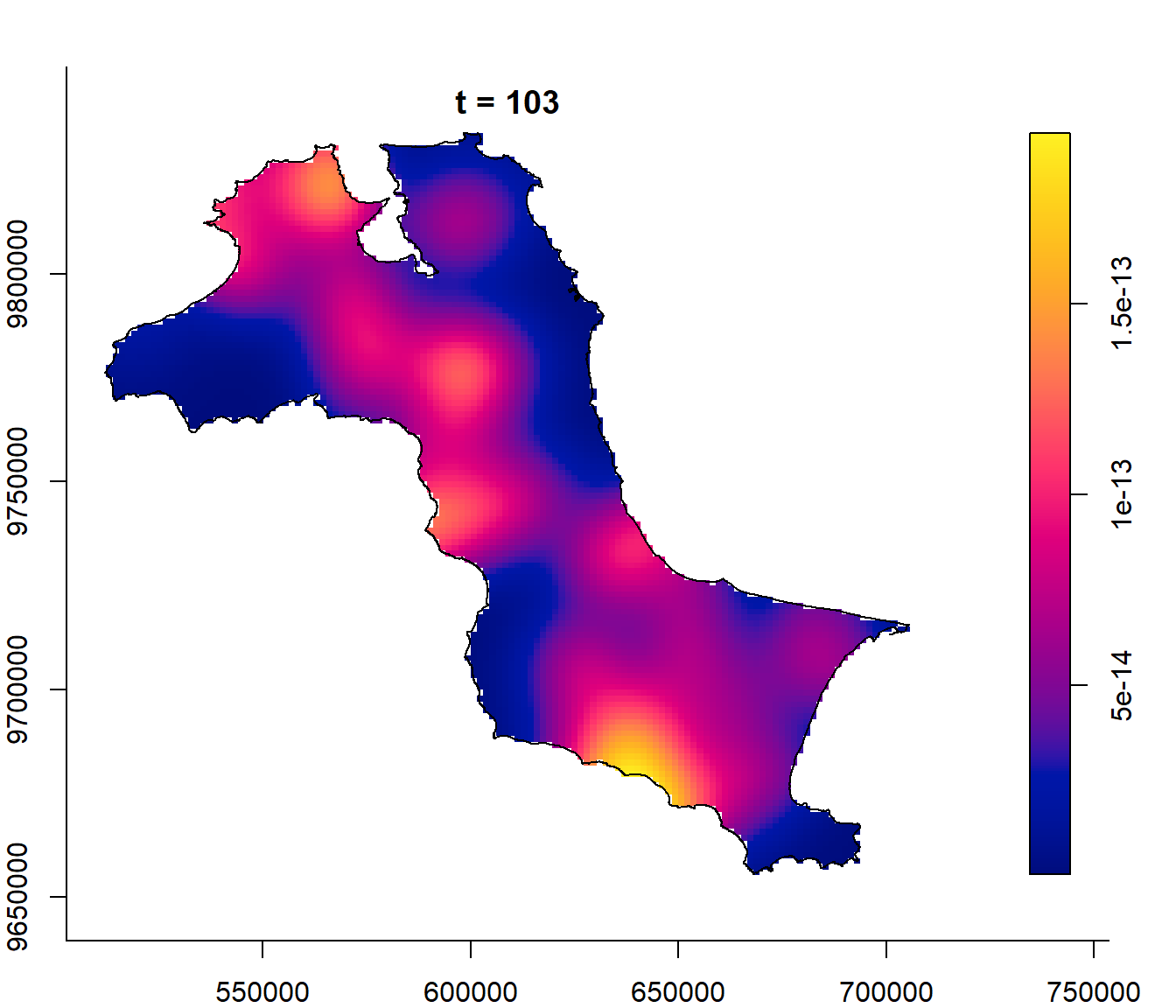
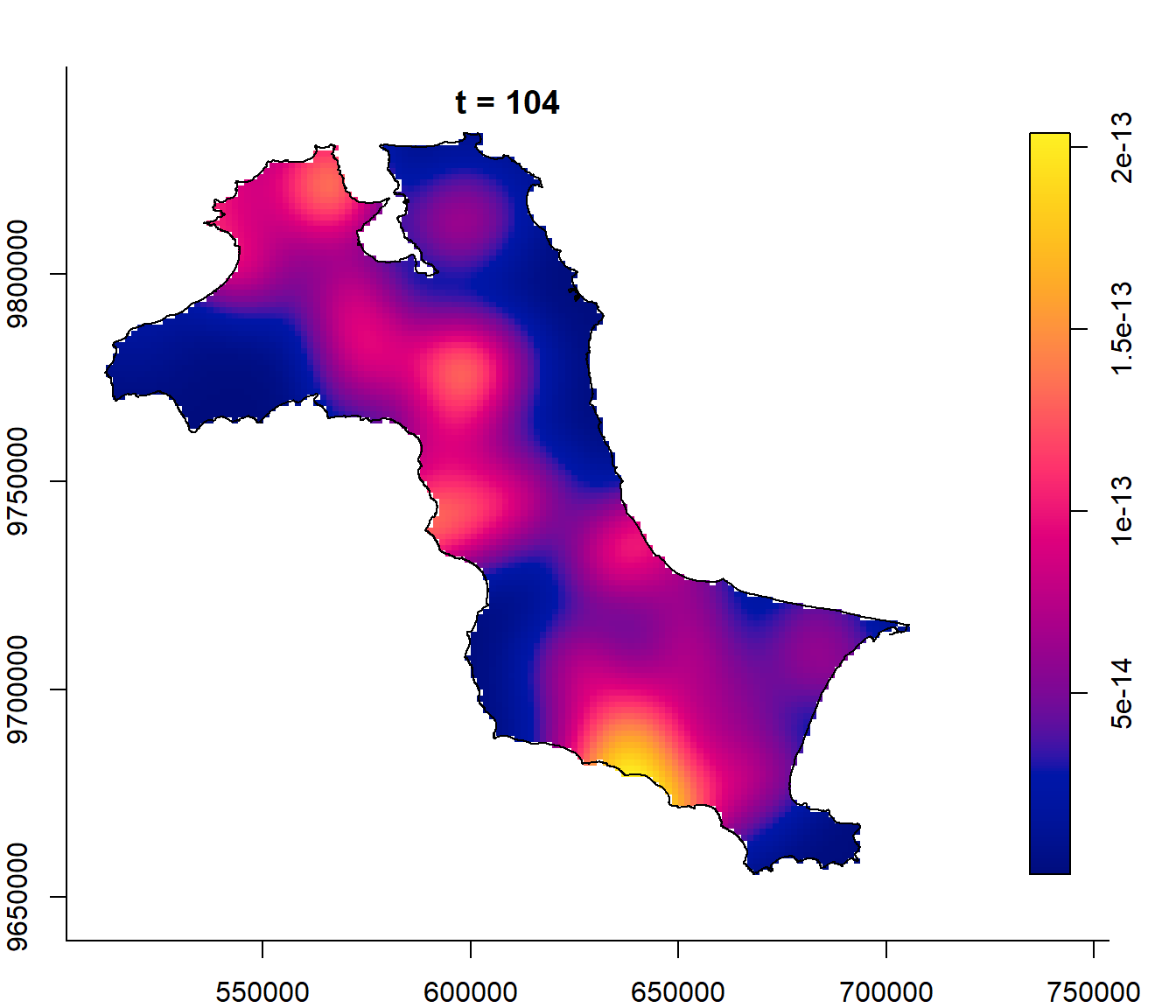
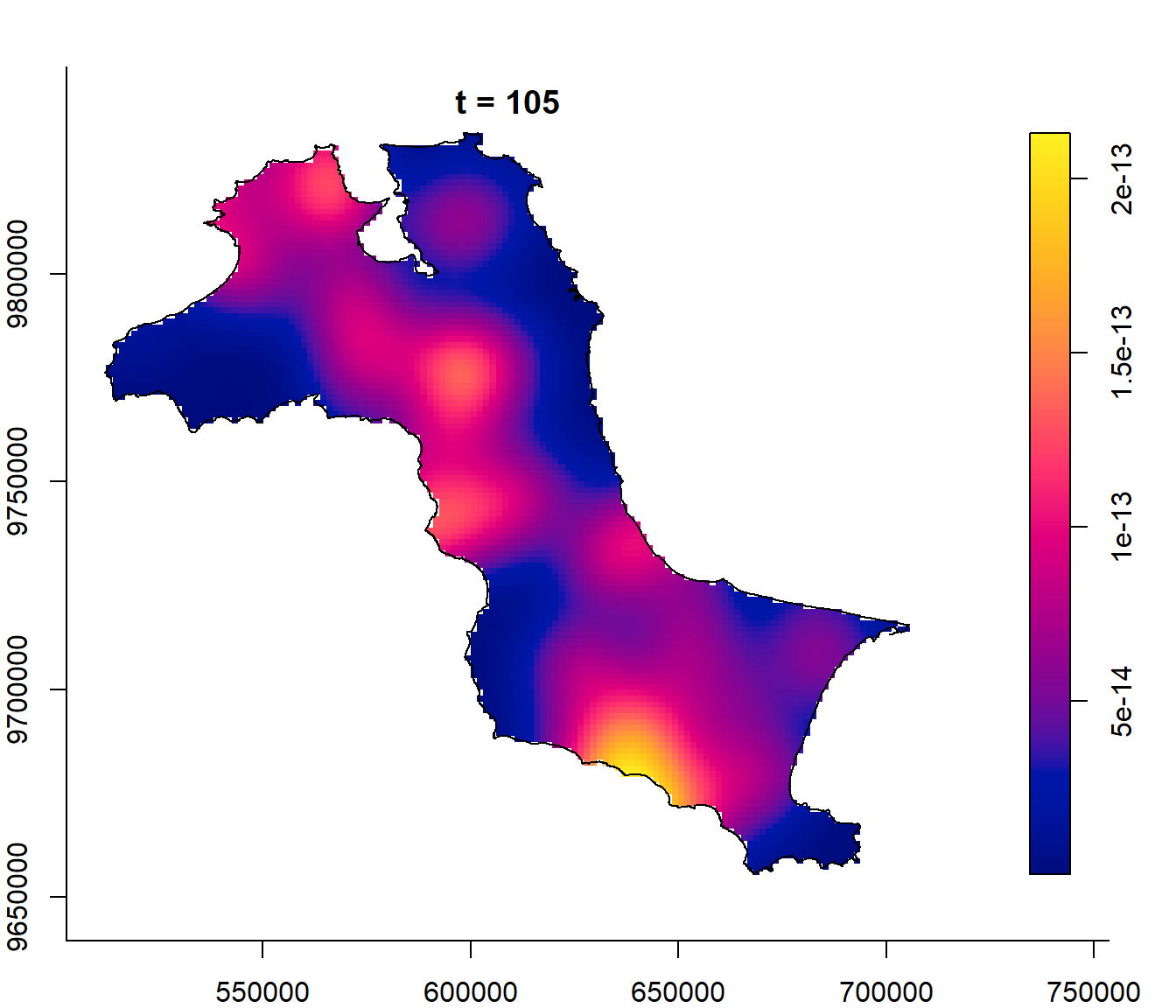
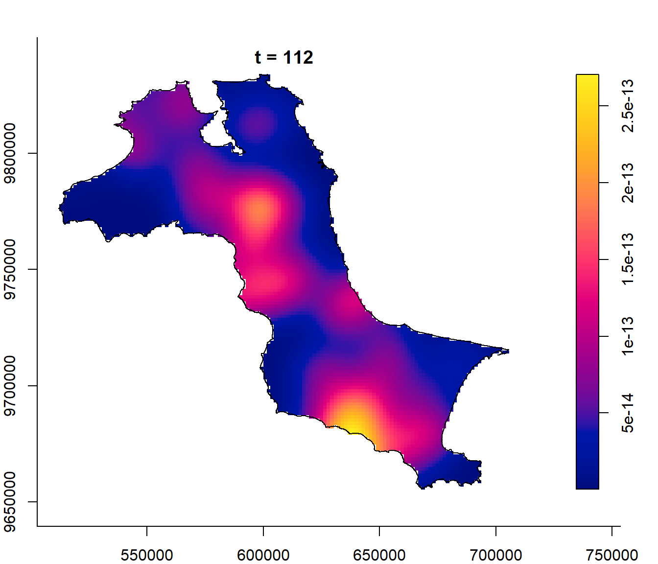
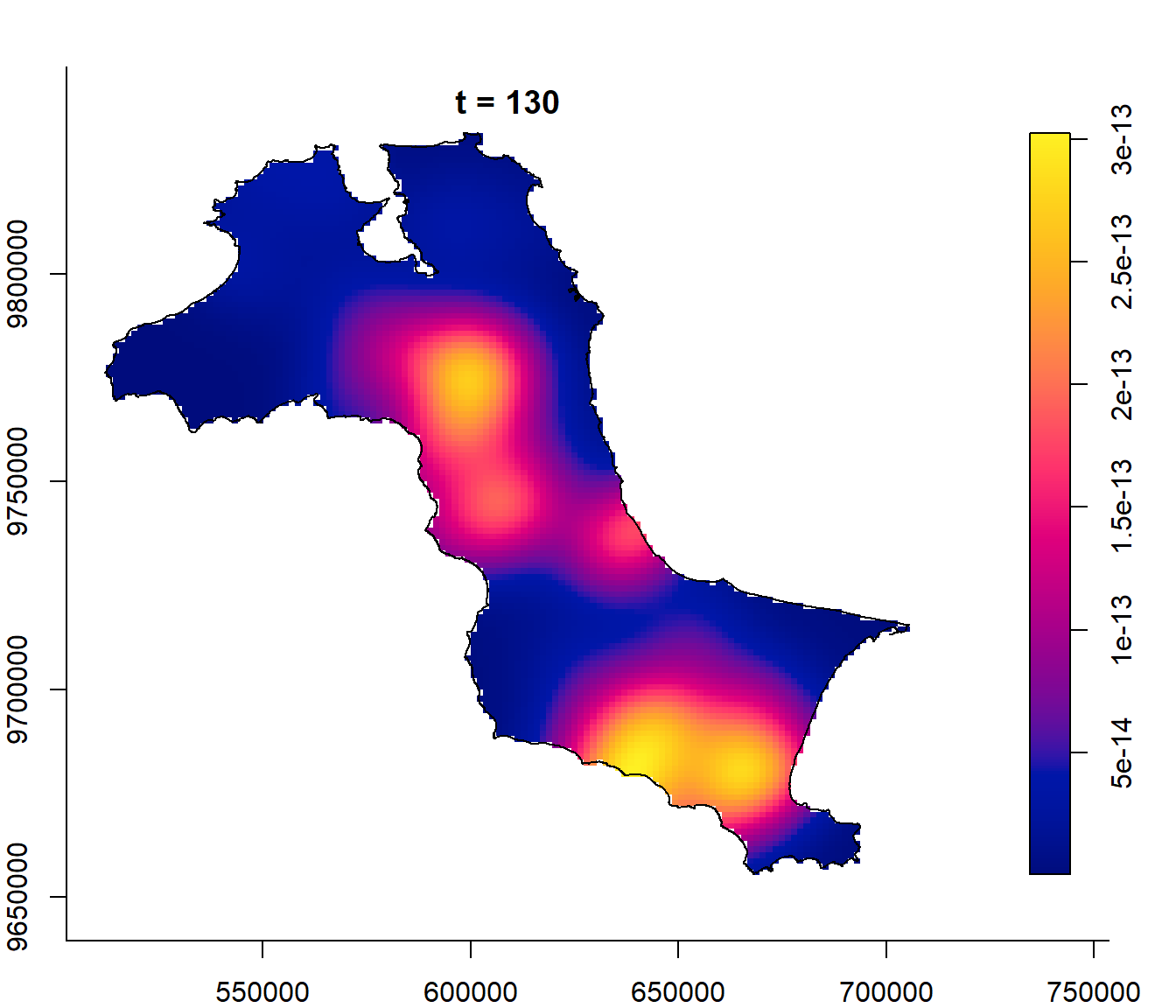
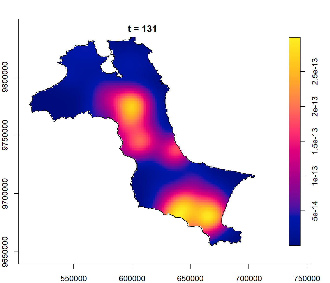
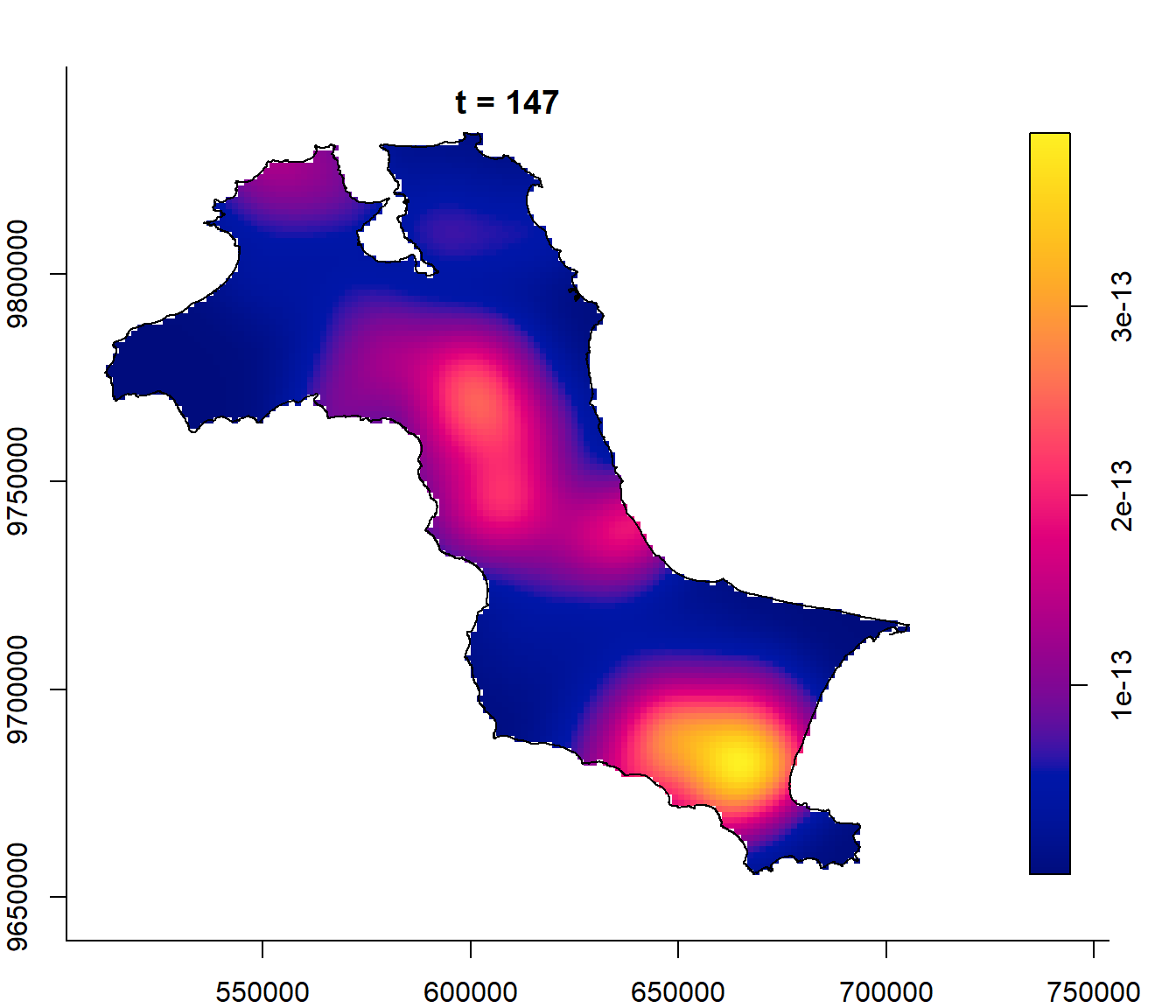
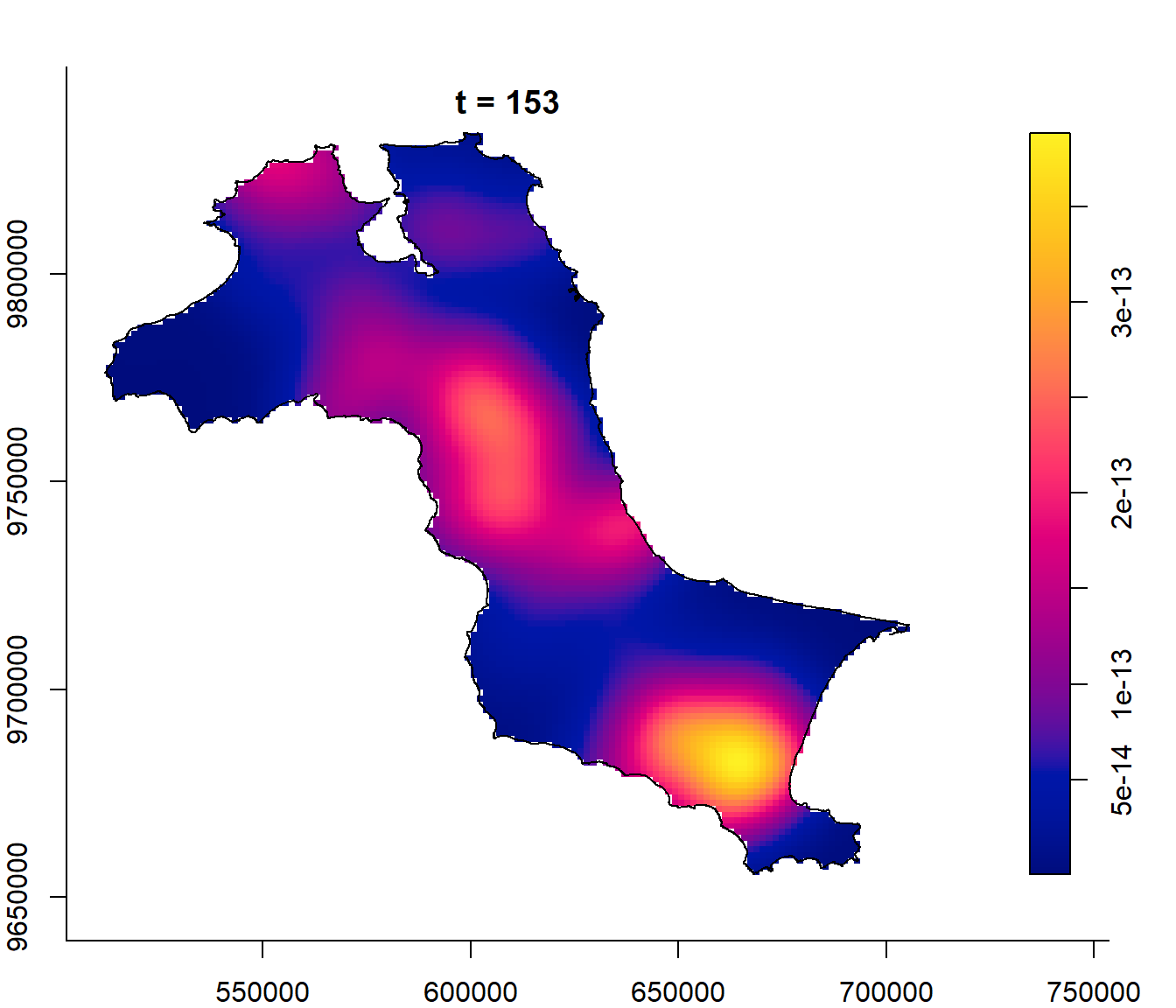
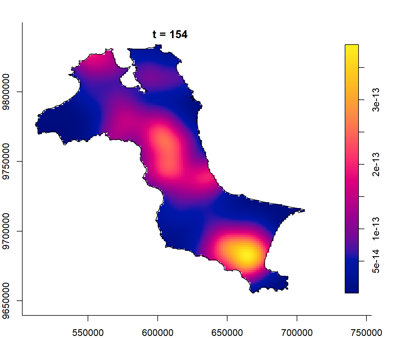
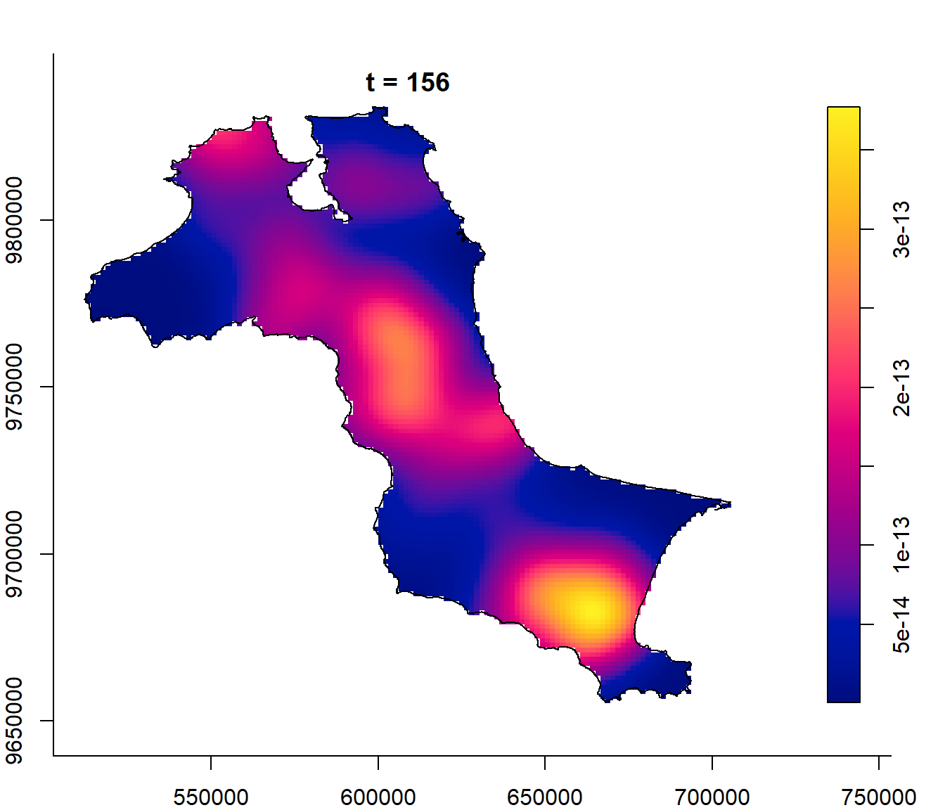
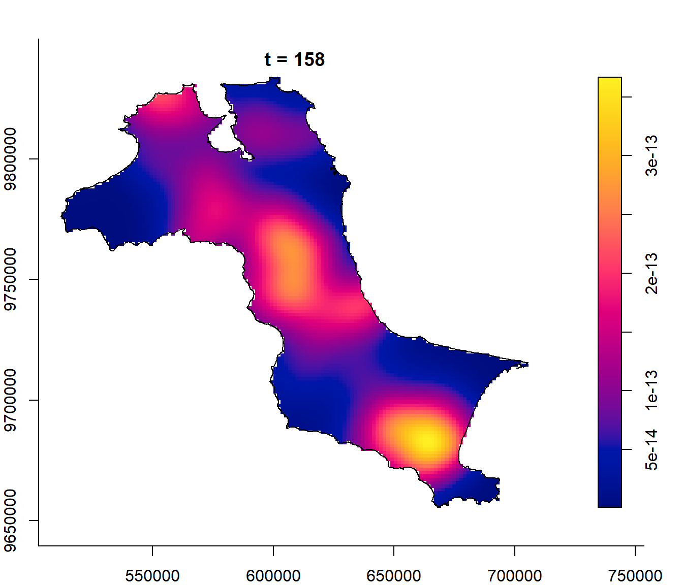
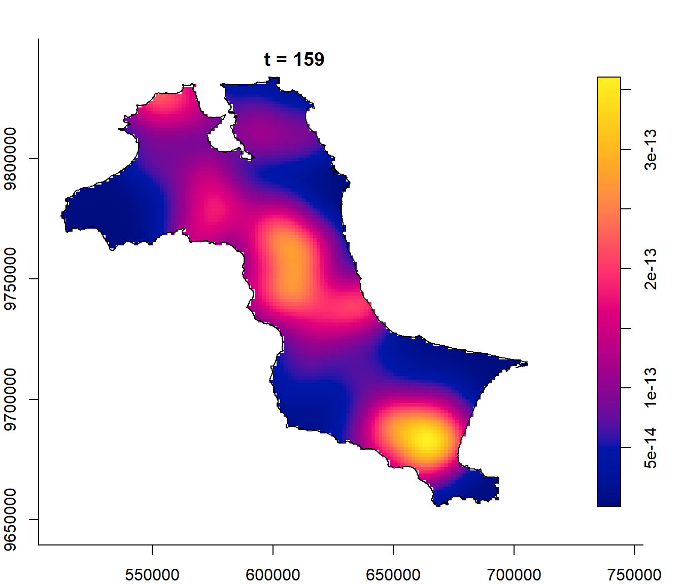
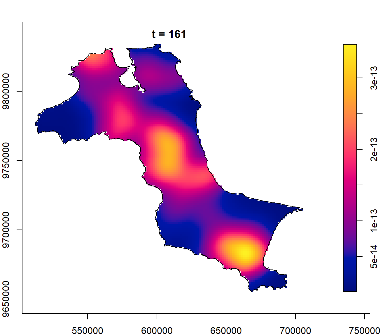
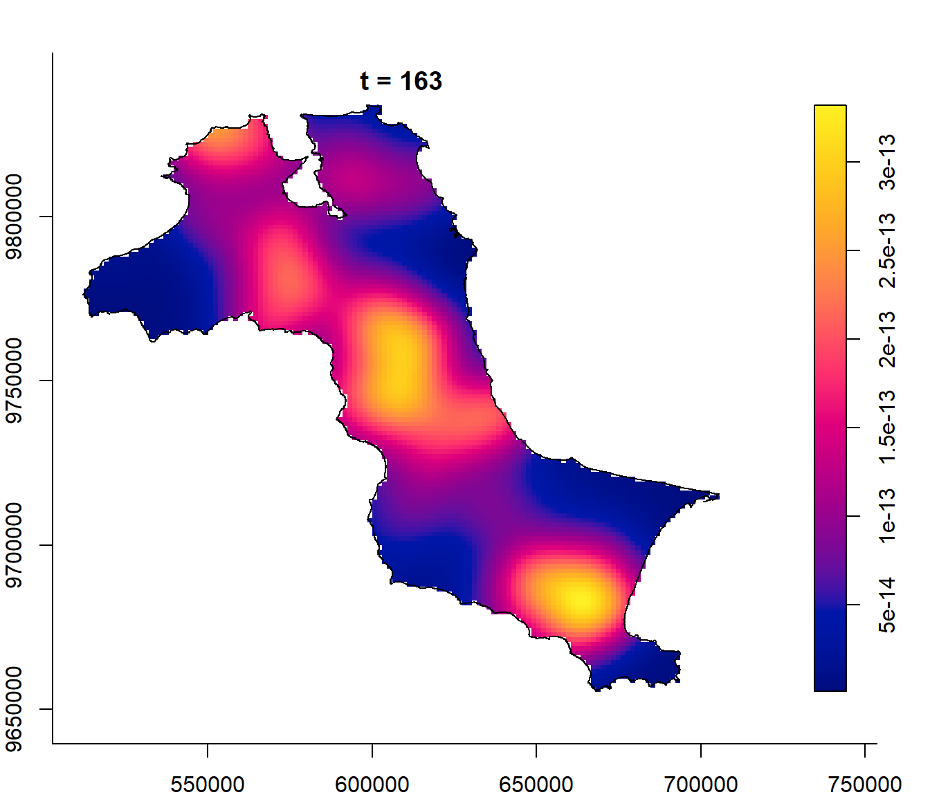
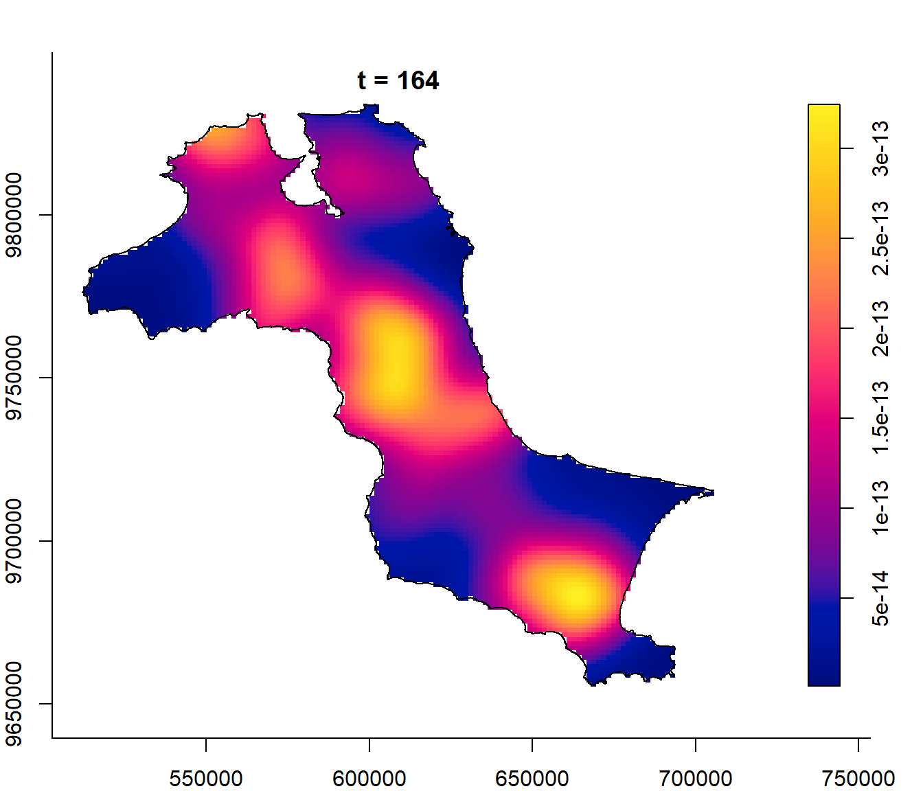
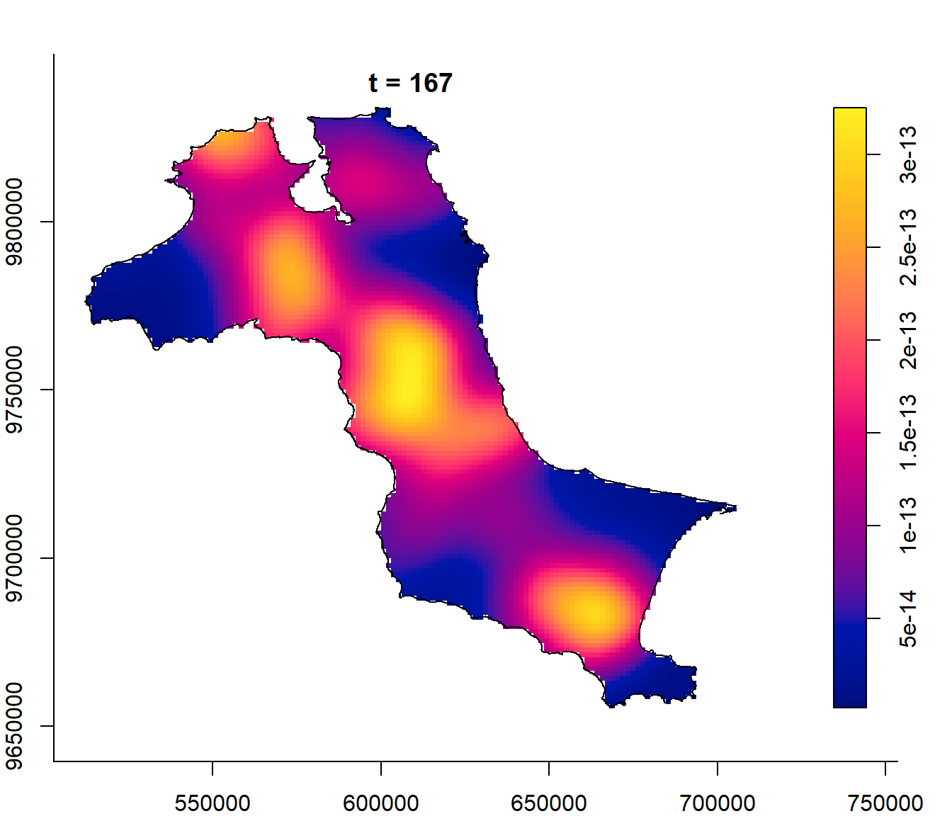
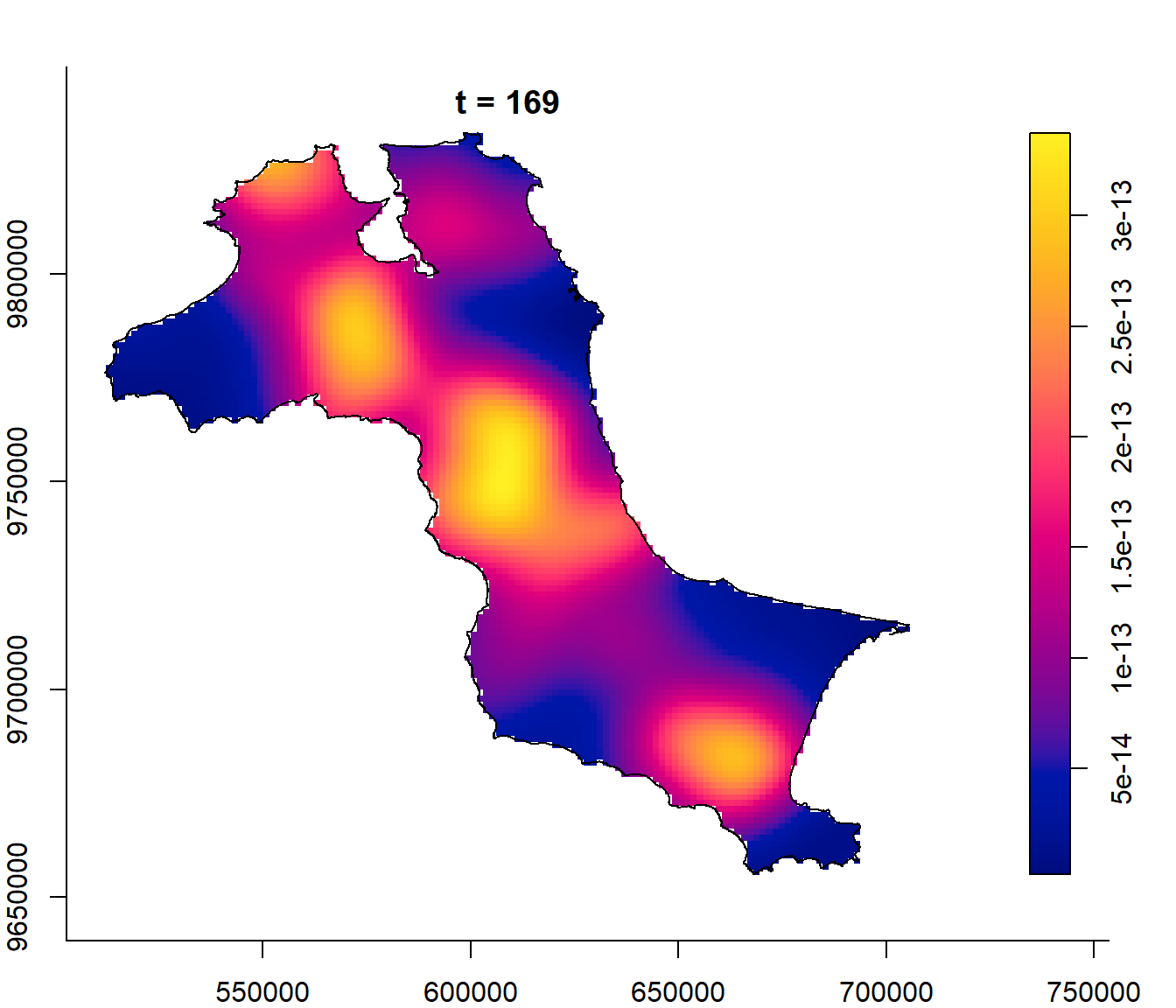
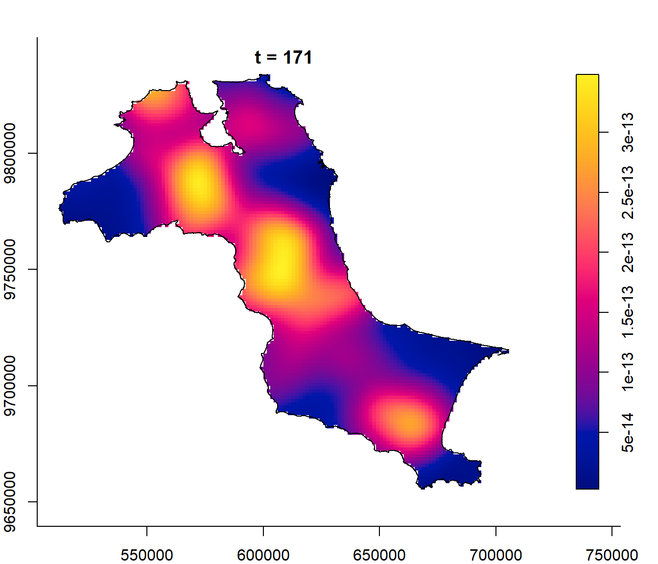
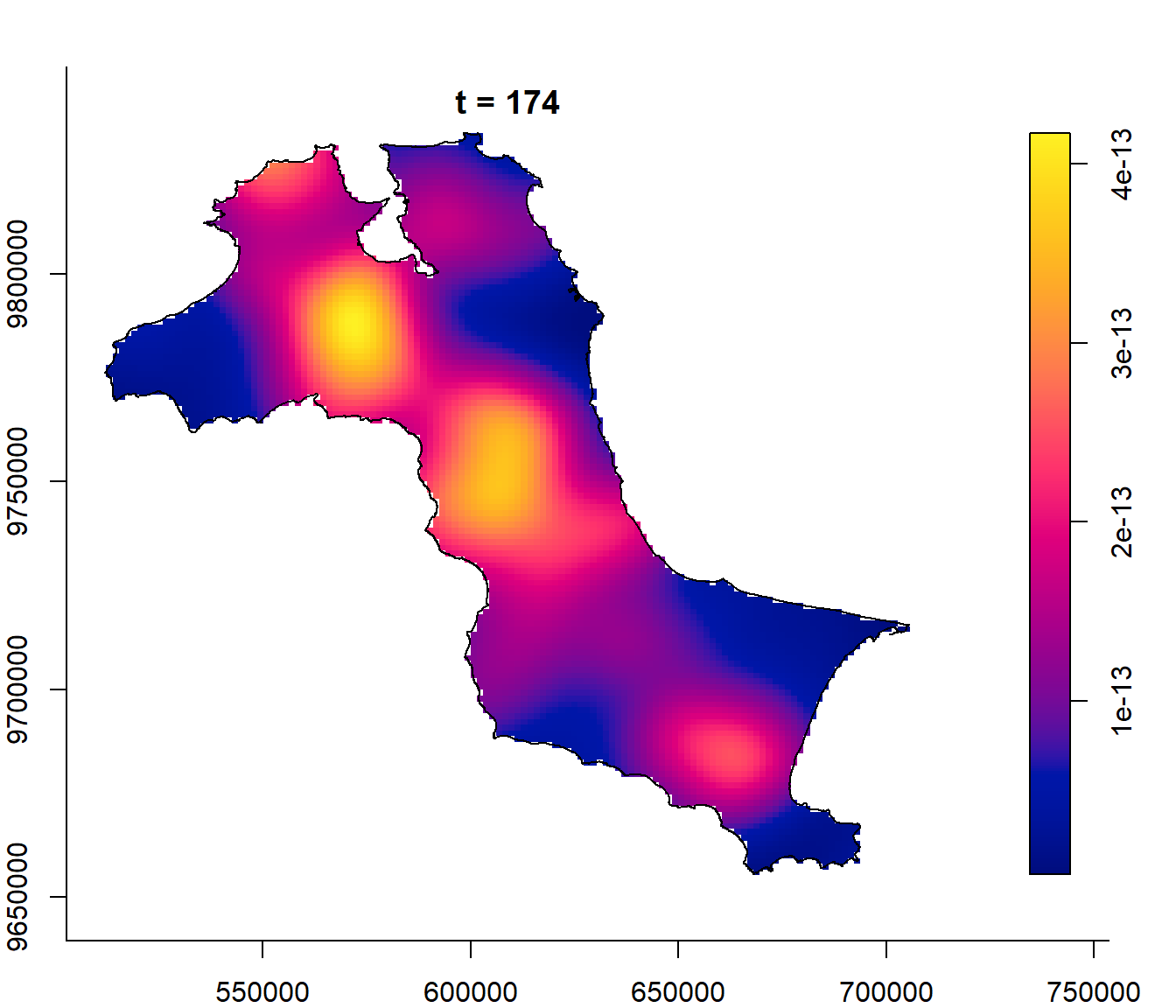
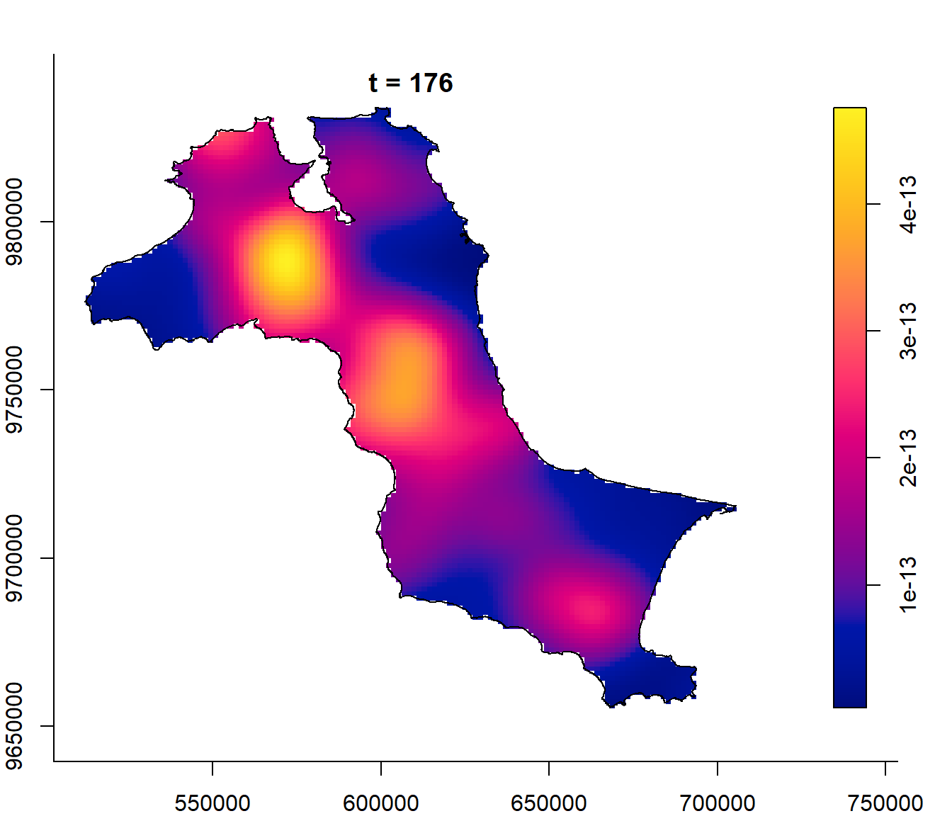
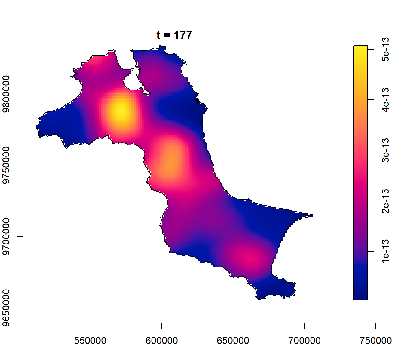
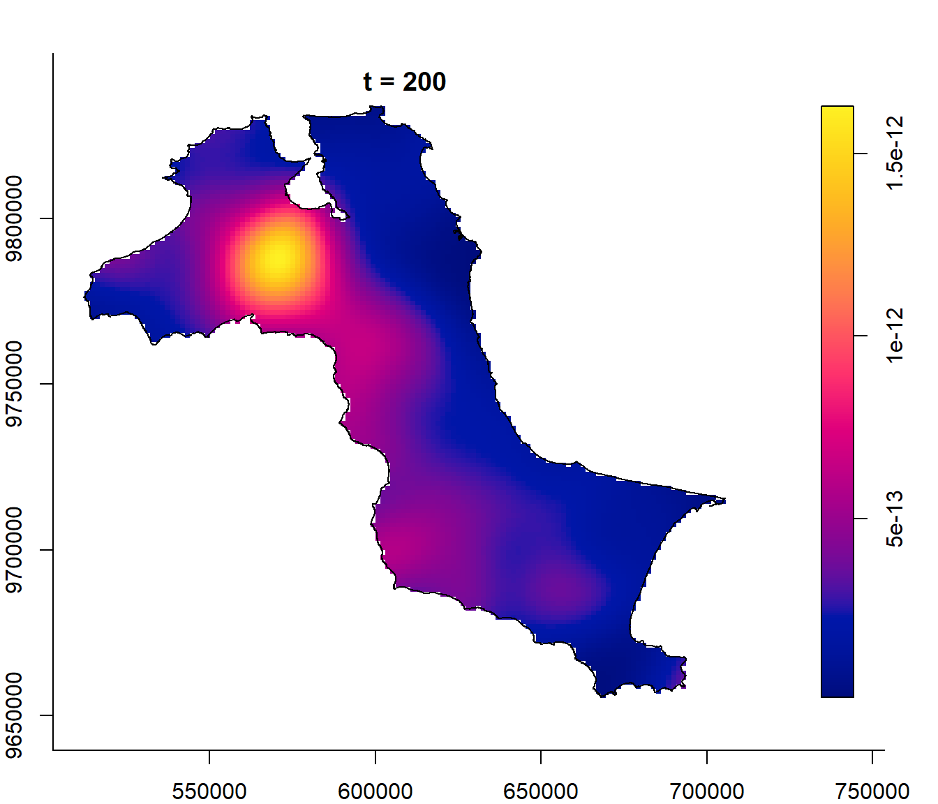
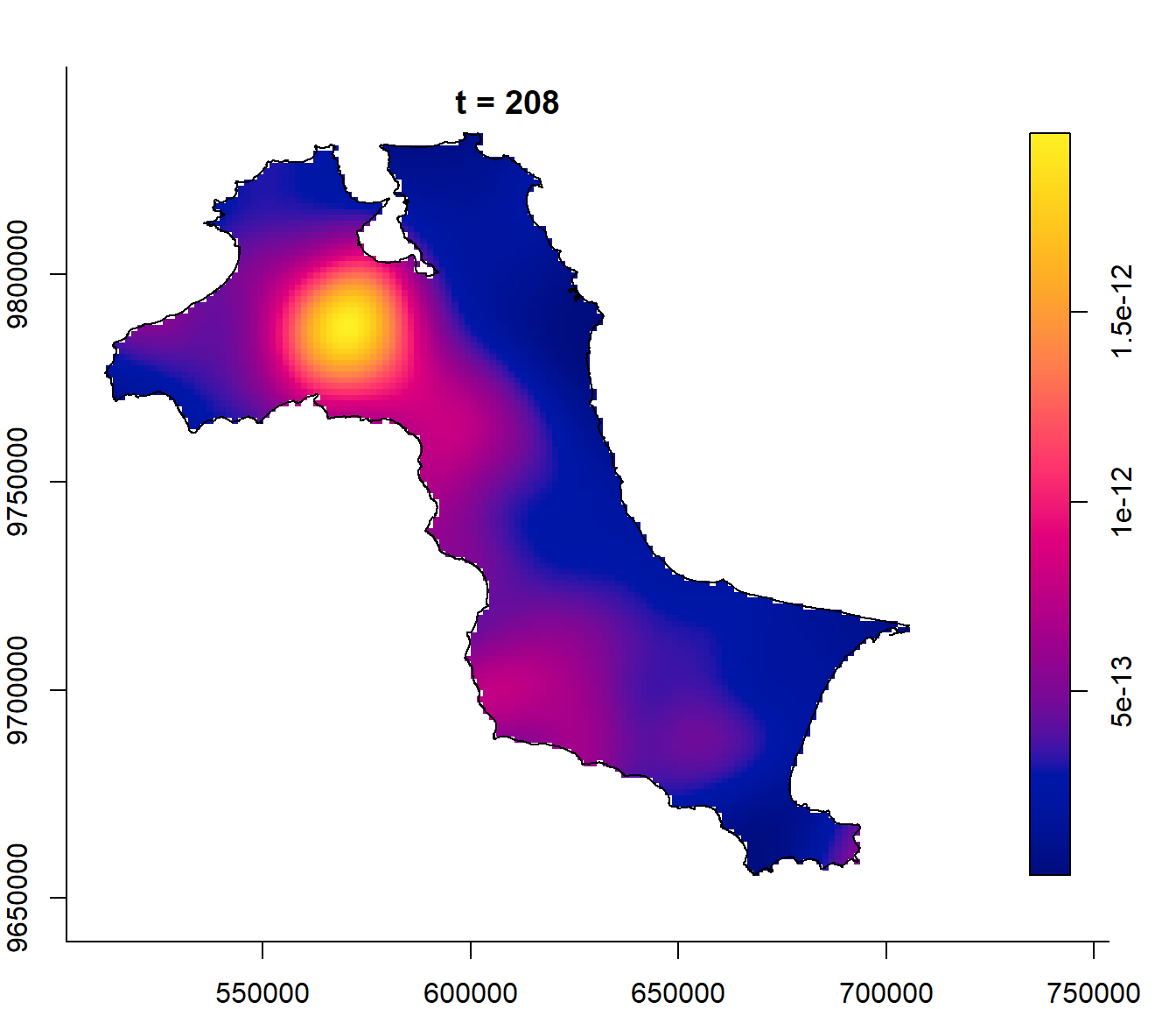
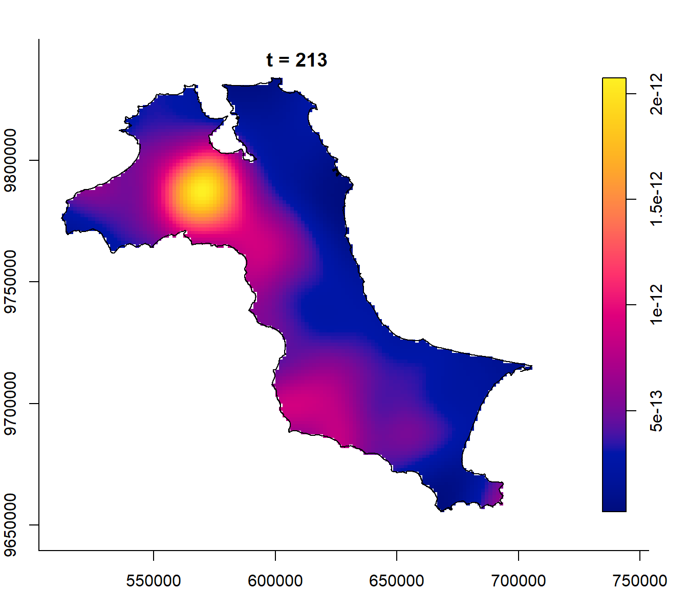
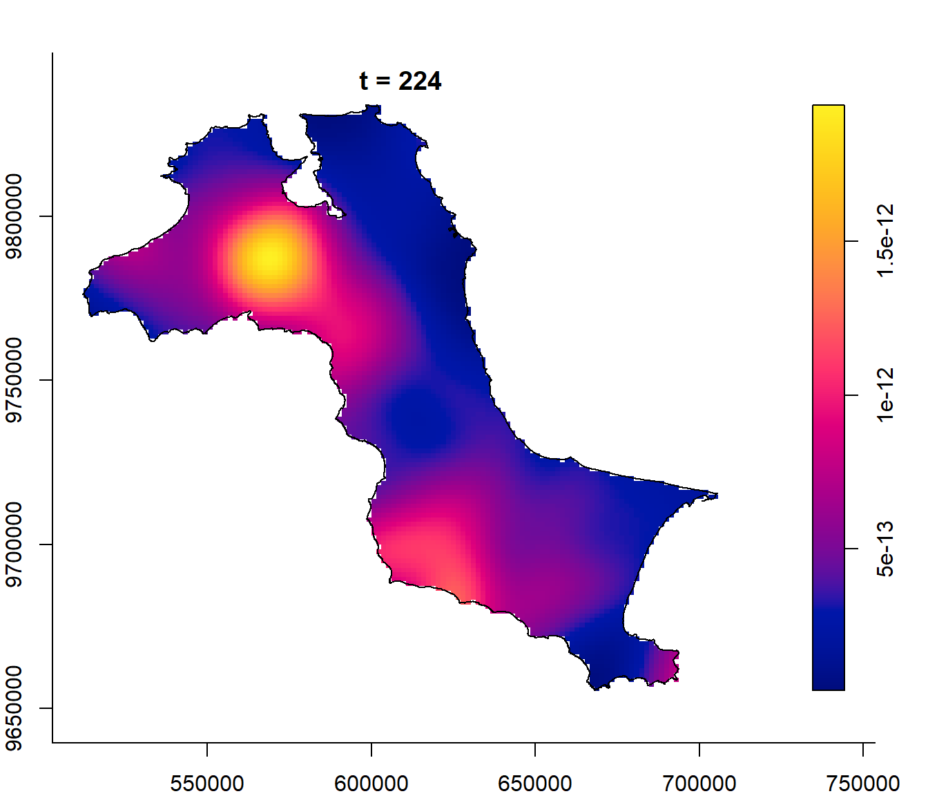
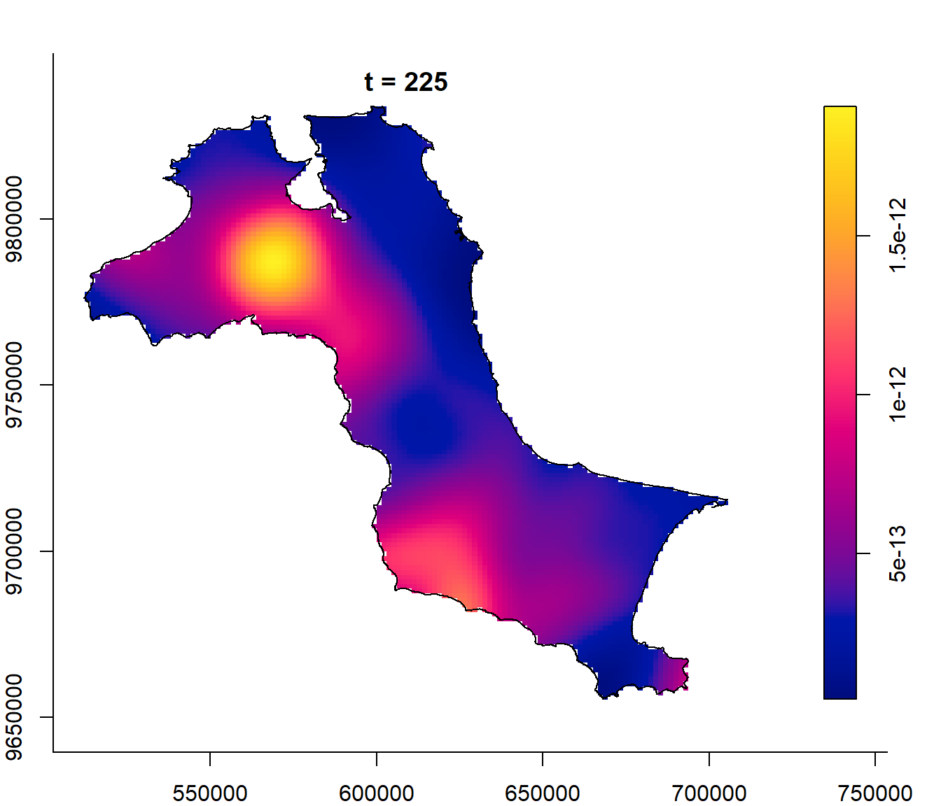
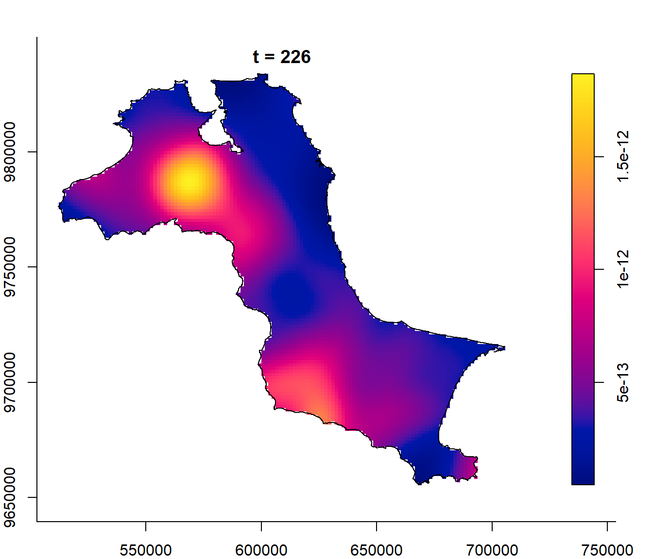
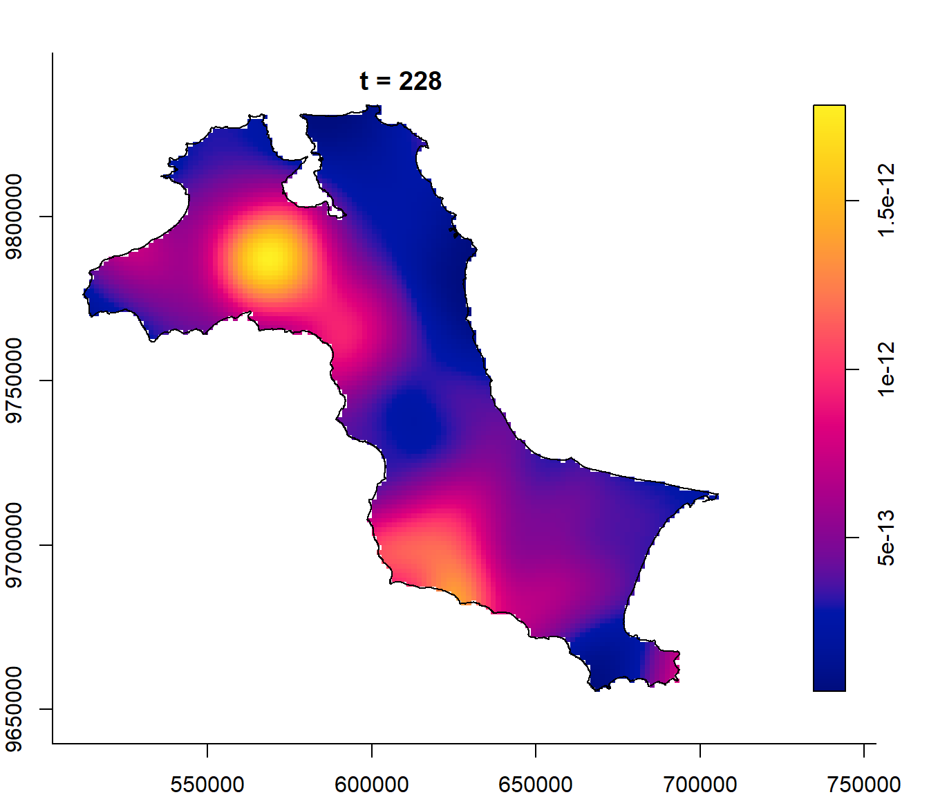
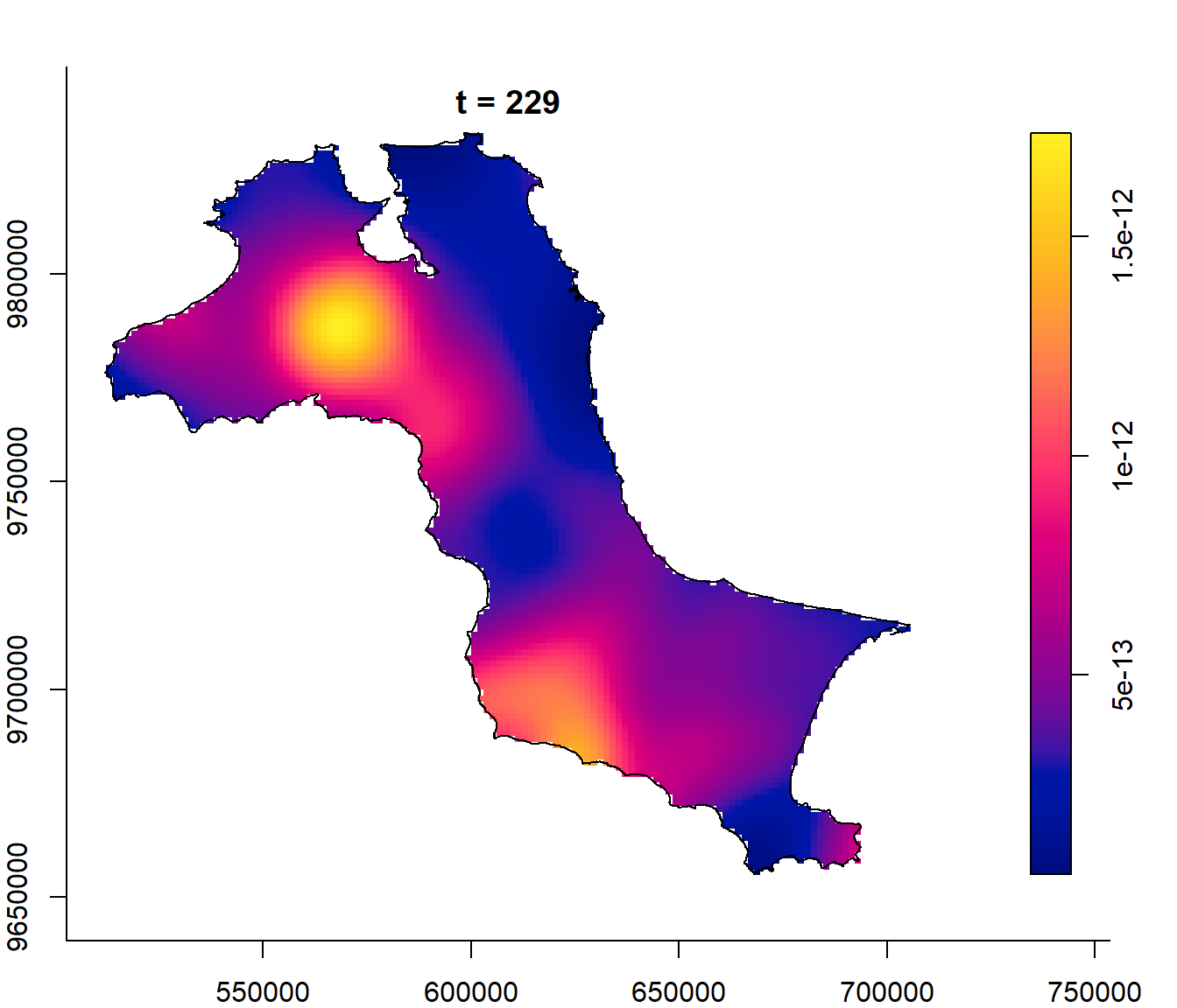
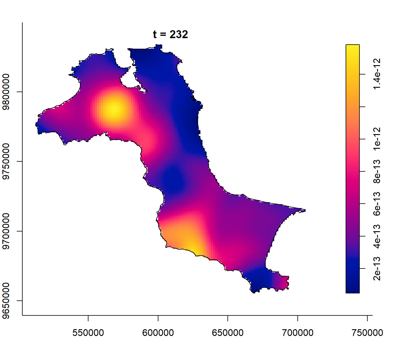
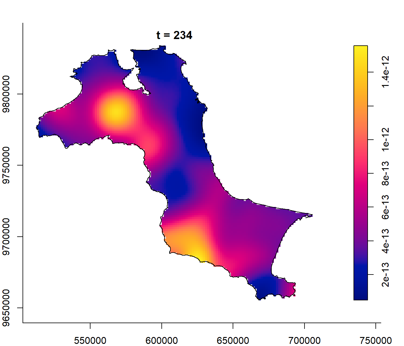
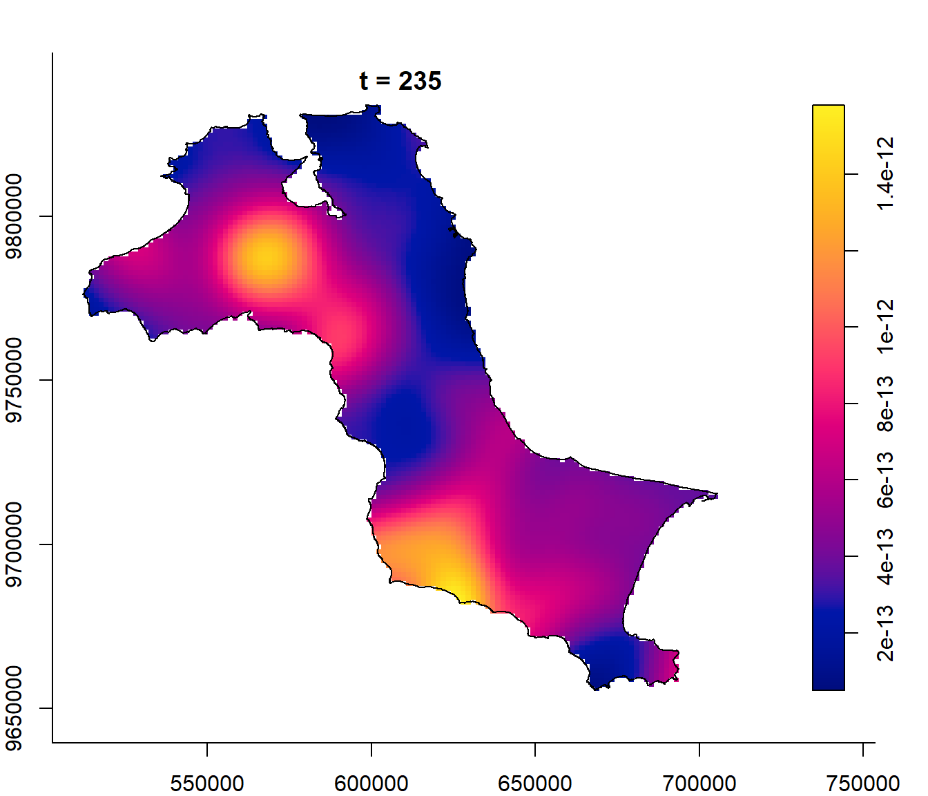
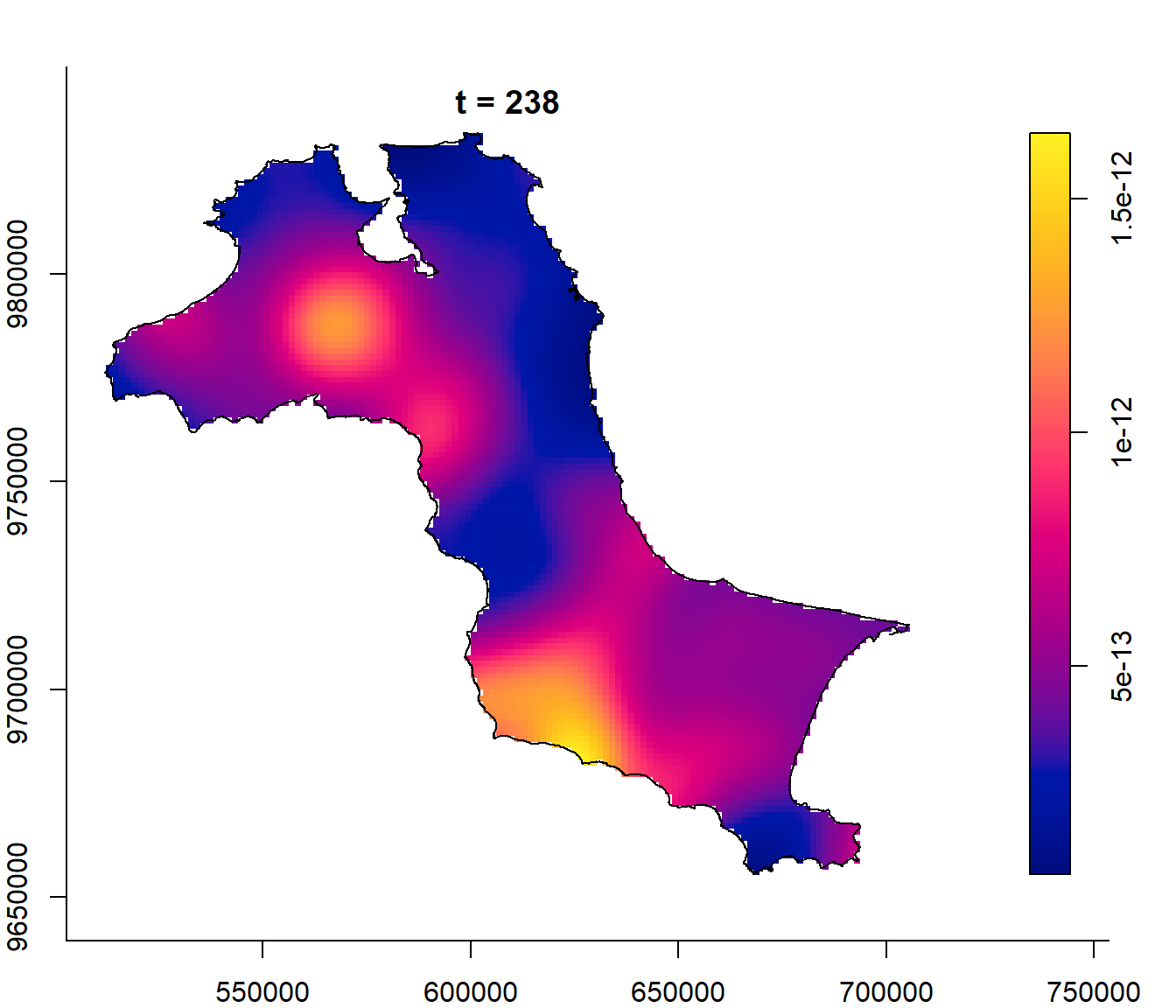
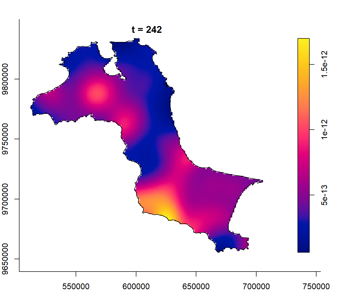
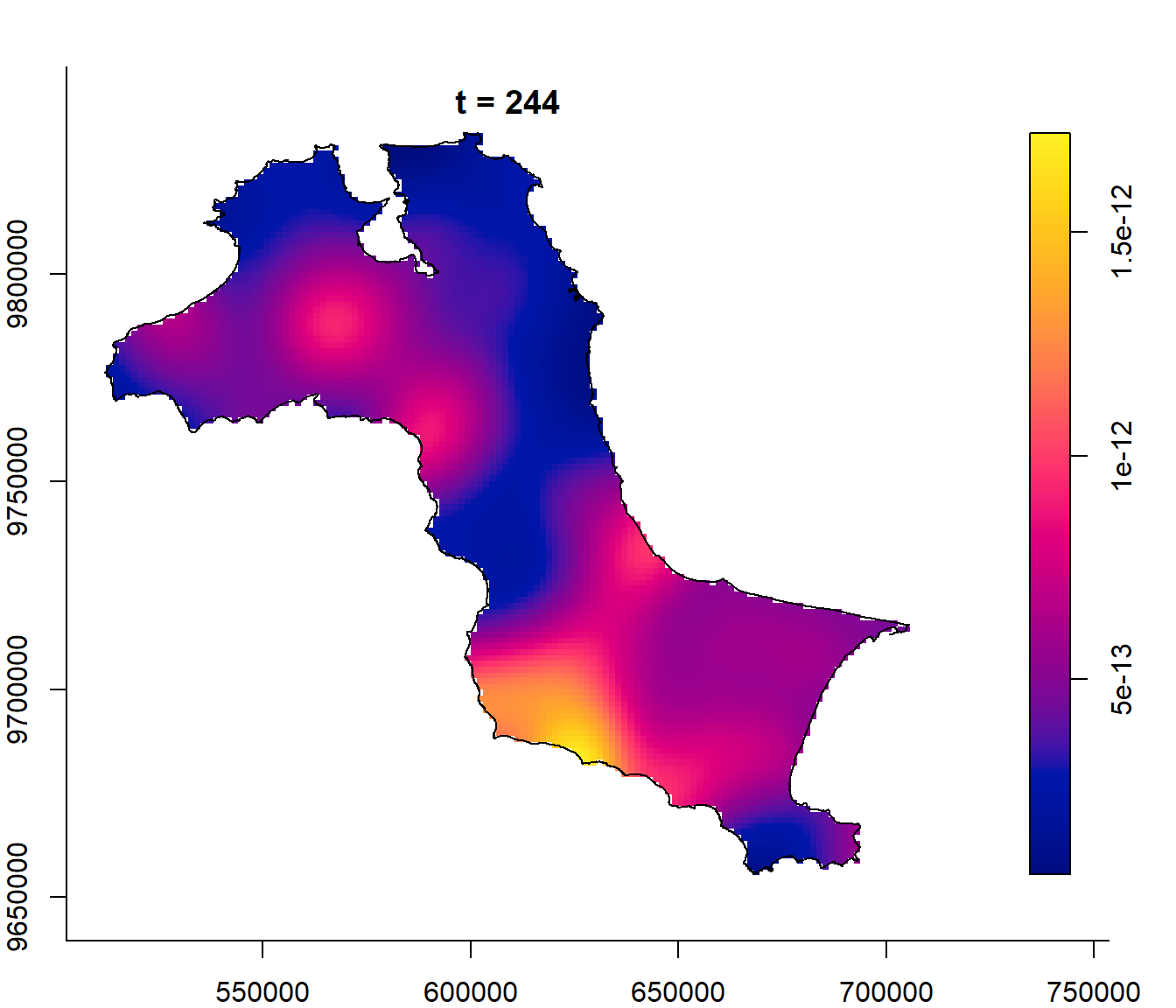
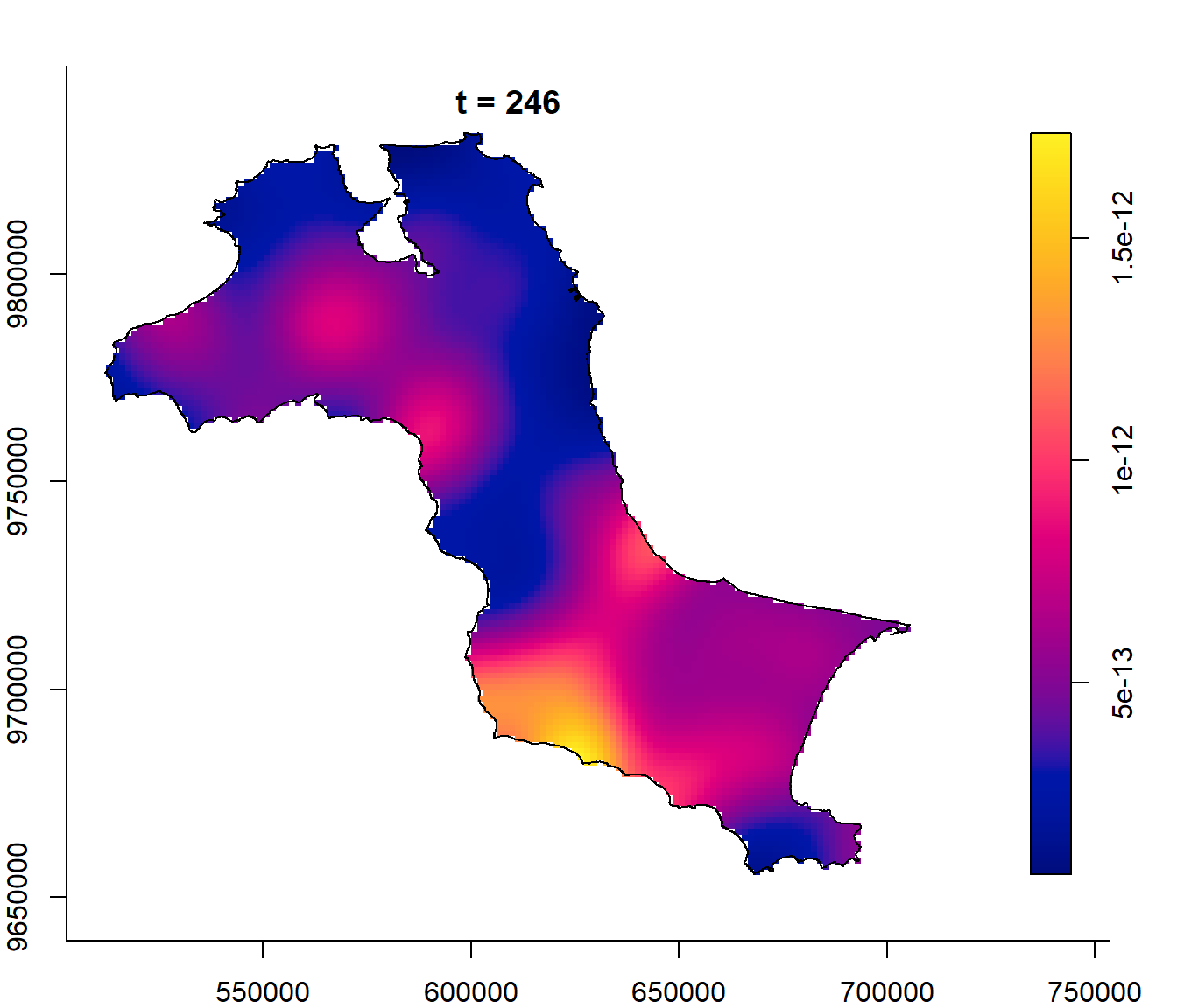
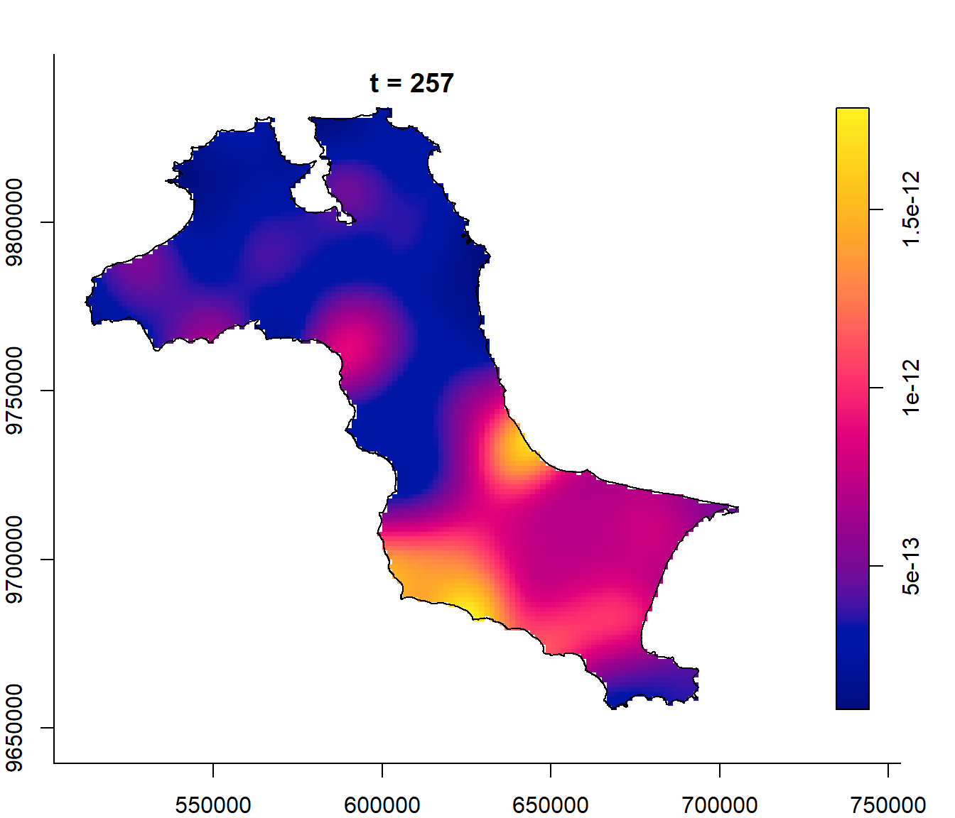
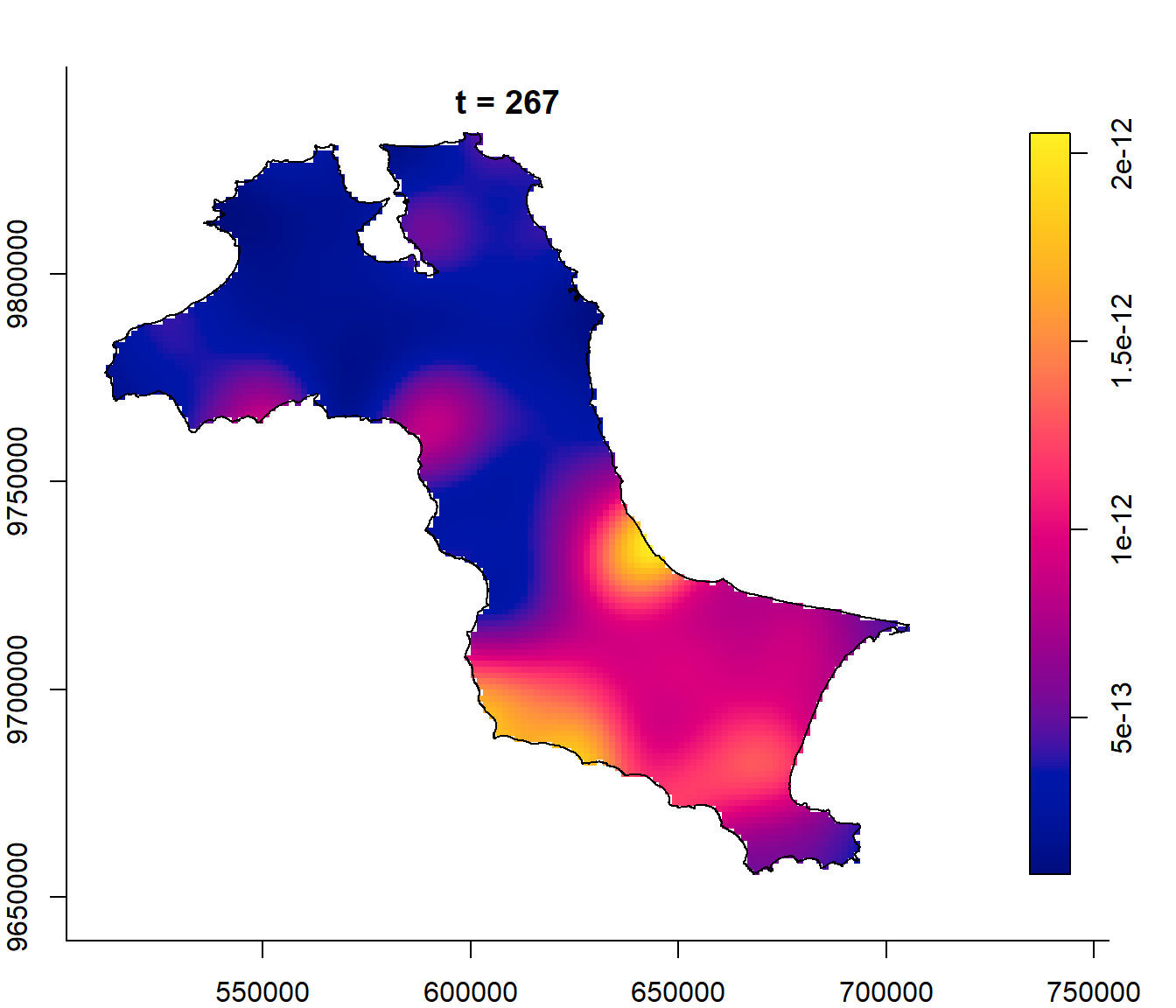
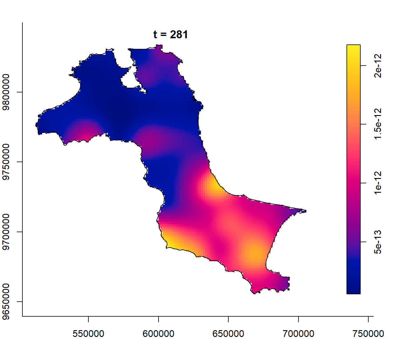
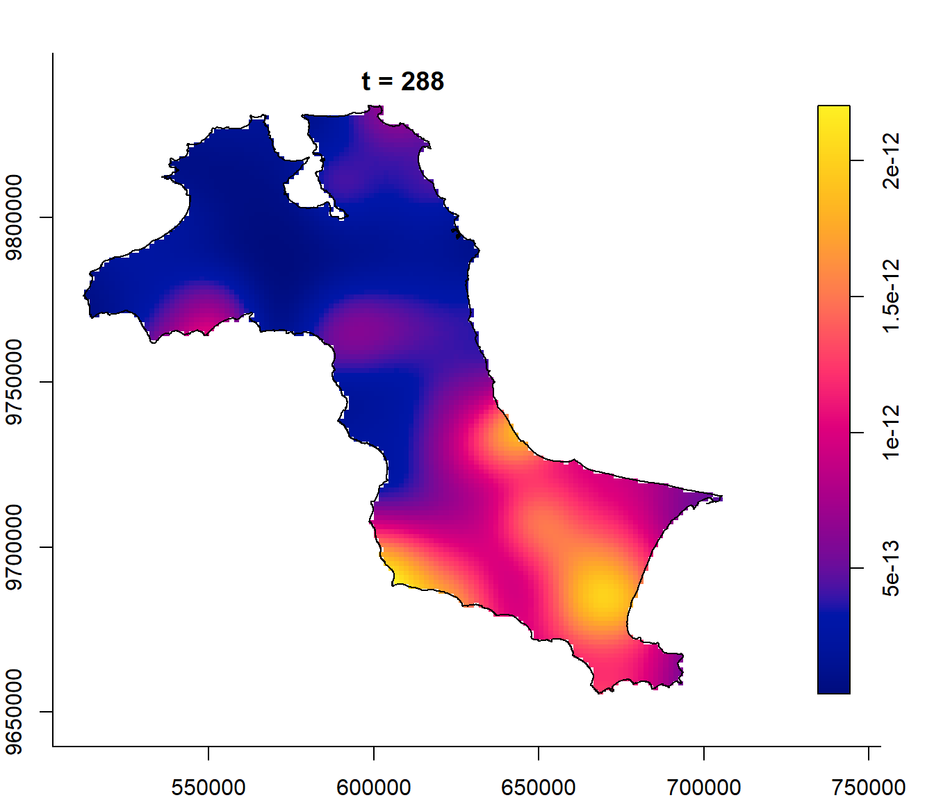
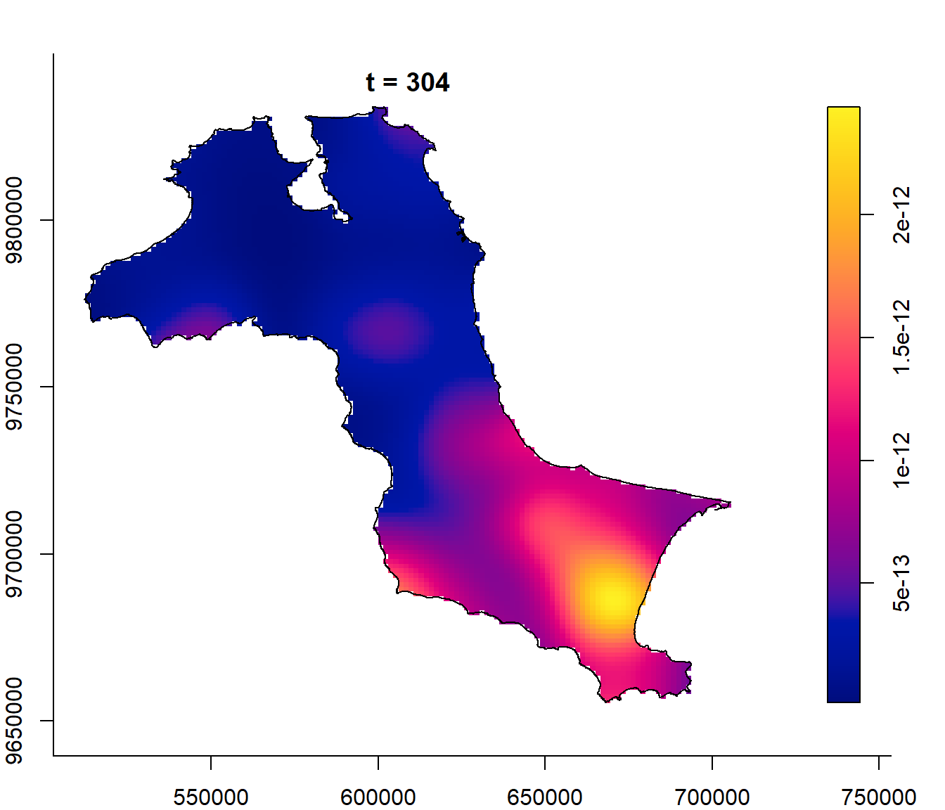
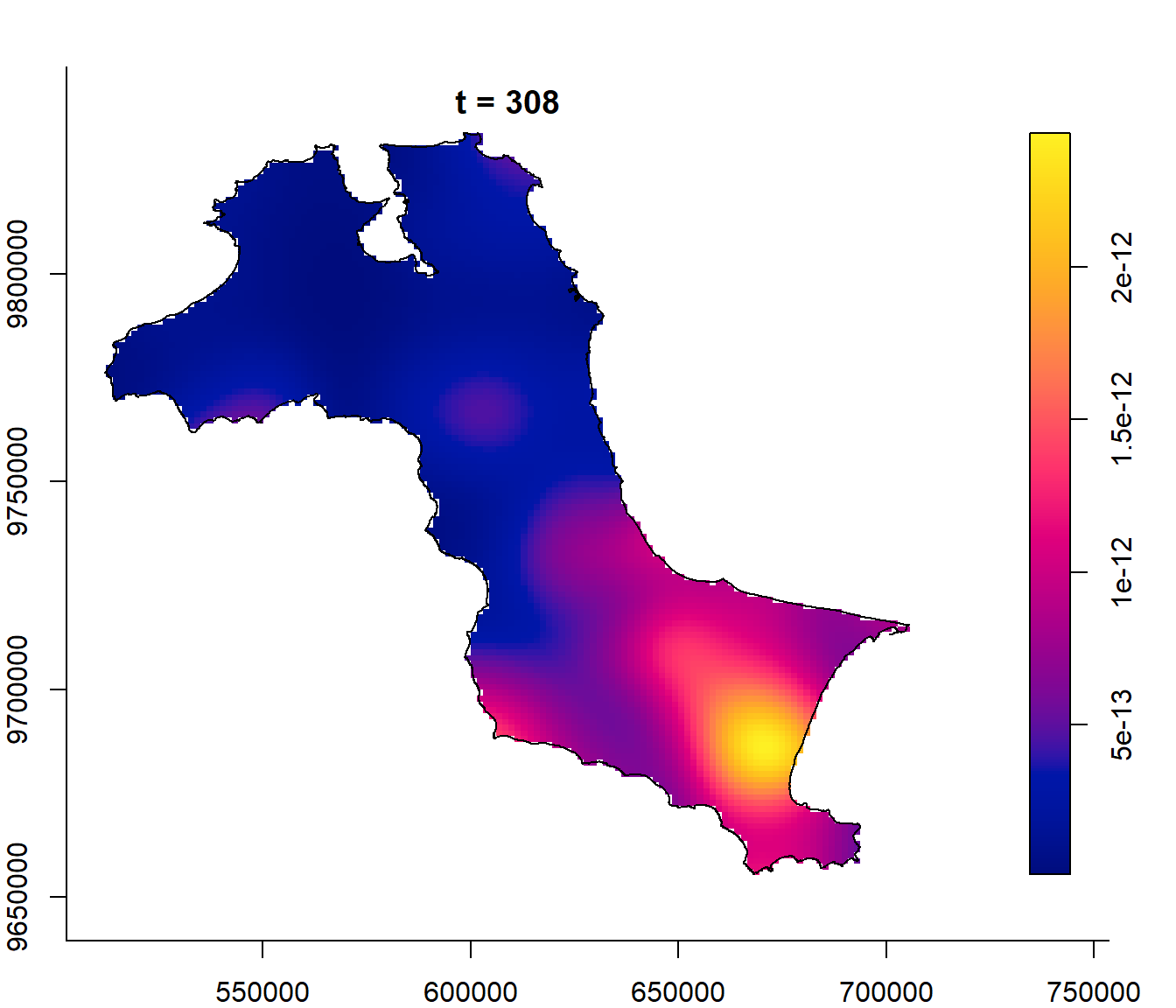
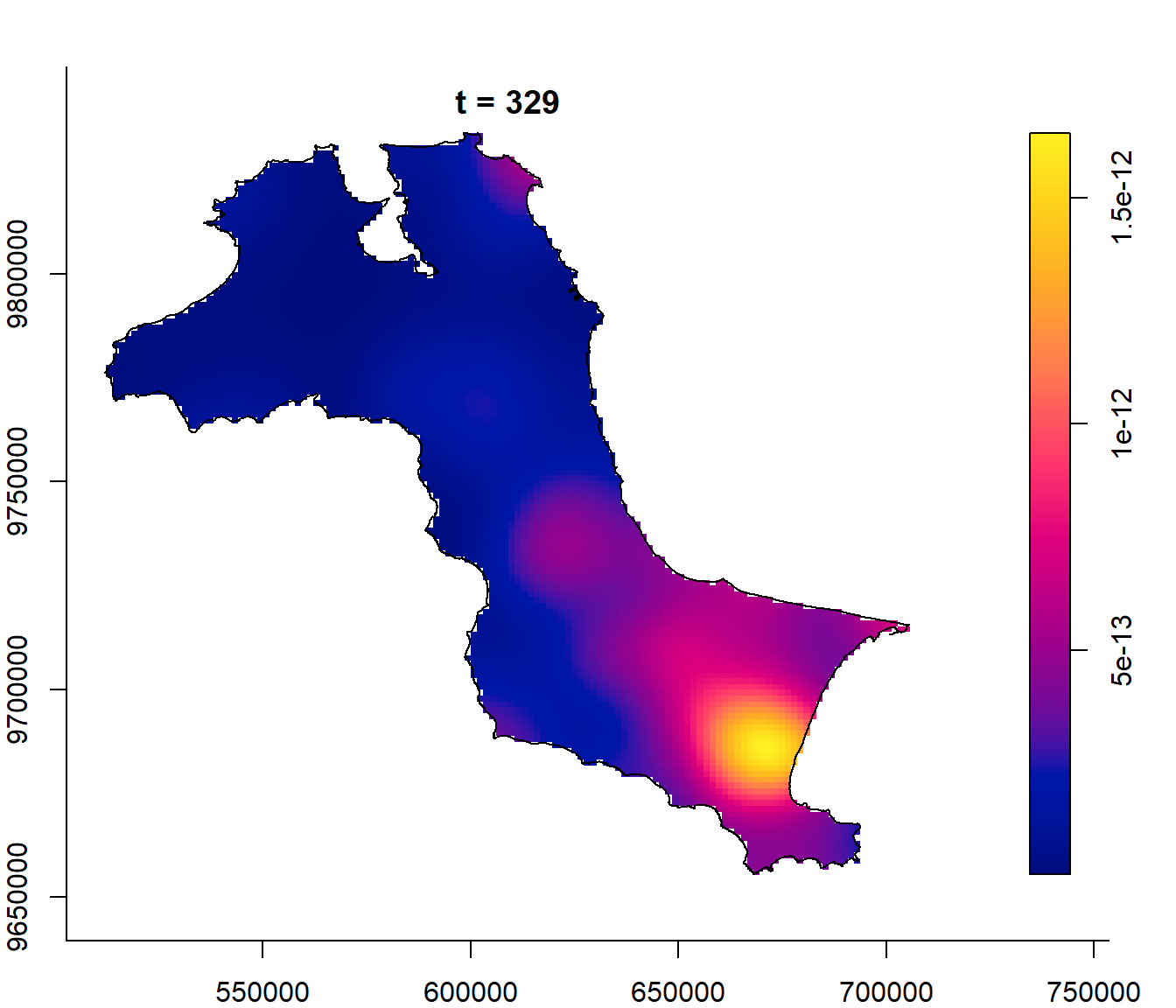
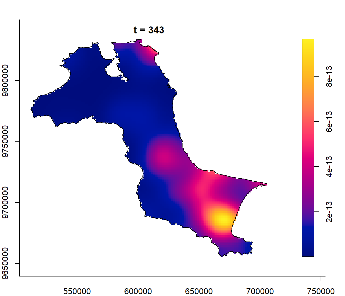
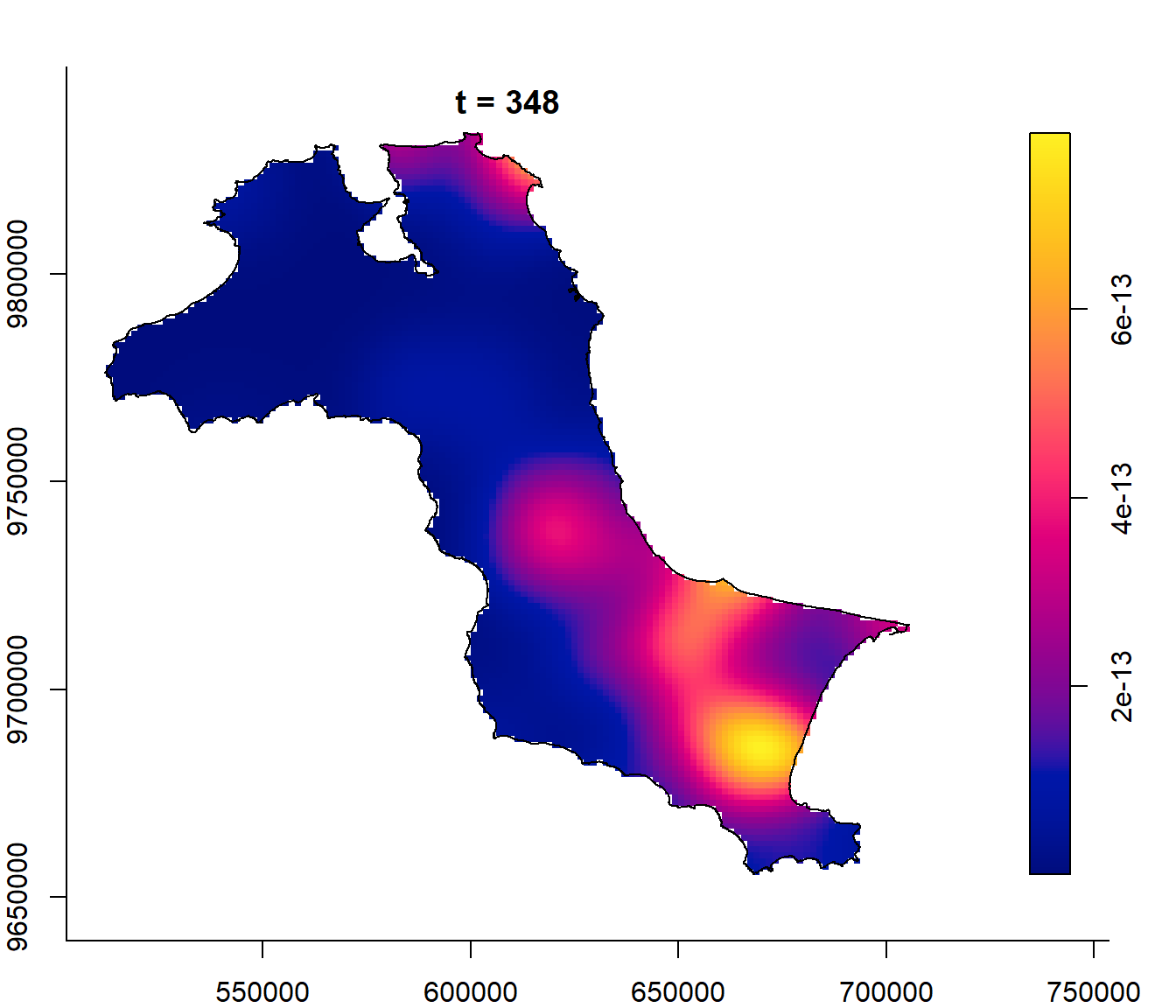
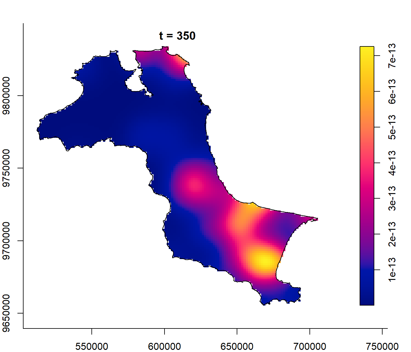
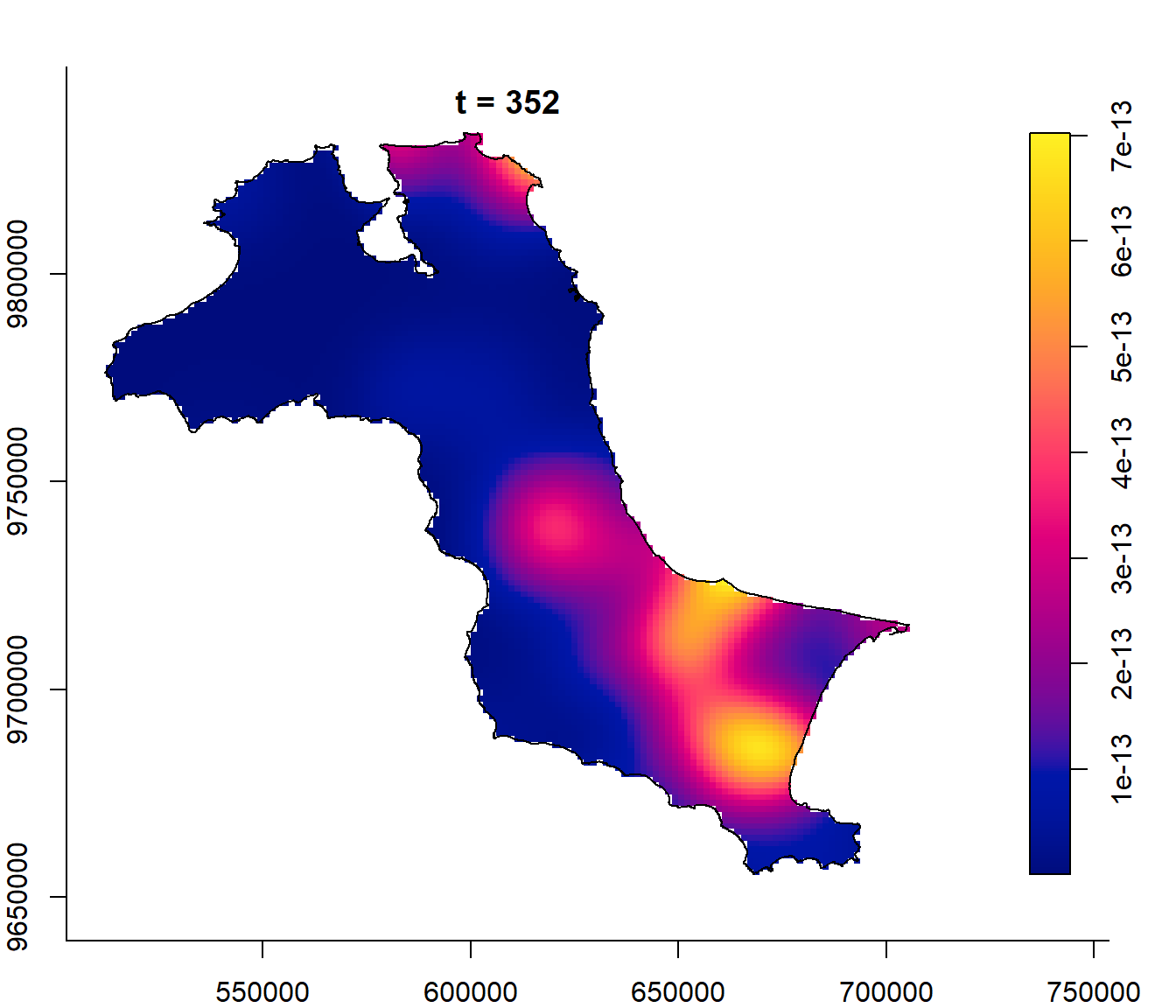
Density range: [2.001642e-19, 2.445724e-12]6.10.2 Plotting the output spatio-temporal KDE
Last, plot() of sparr package is used to plot the output as shown below.
plot(kde_yday)


6.11 Spatio-temporal Point Patterns Analysis: stpp methods
In this section, you will gain hands-on experience on using functions of stpp package to perform spatio-temporal point patterns analysis.
Students are encouraged to read stpp: An R Package for Plotting, Simulating and Analyzing Spatio-Temporal Point Patterns to learn more about the package.
6.11.1 Preparing spatio-temporal point process object of stpp
Step 1: Extracting forest fire coordinates from the fire point events
coords <- st_coordinates(fire_sf)Step 2: Creating a data frame by combining the x- and y-coordinates and temporal event. Note that the temporal event must be in integer.
fire_df <- data.frame(
  x = coords[, 1],
  y = coords[, 2],
  t = fire_sf$`DayofYear`)
Step 3: Creating stpp spatio-temporal object
In the code chunk below, as.3dpoint() of stpp package is used to create stpp spatio-temporal object class.
fire_stpp <- as.3dpoints(fire_df)Use the code chunk below to confirm that the output is in stpp spatio-temporal object class.
class(fire_stpp)[1] "stpp"Next we can visual fire_stpp by using the code chunk below.
plot(fire_stpp)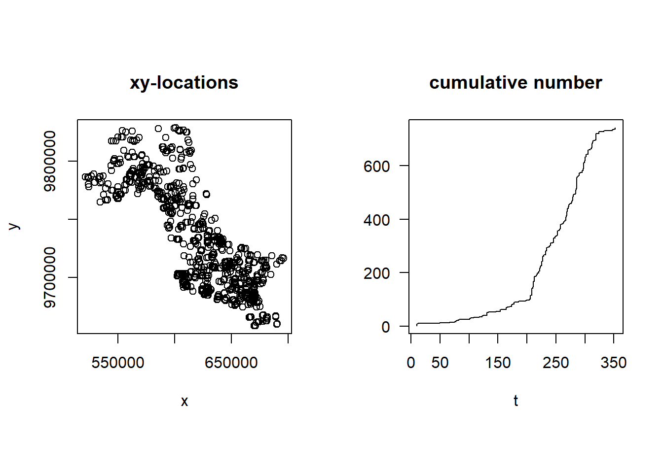
6.11.2 Computing spatio-temporal k-function
In the code chunk below, STIKhat() of stpp package is used to compute space-time inhomogeneous K-function.
kbb_stik <- STIKhat(fire_stpp)Next, plotK() is used to visualise the output space-time inhomogeneous K-function.
plotK(kbb_stik)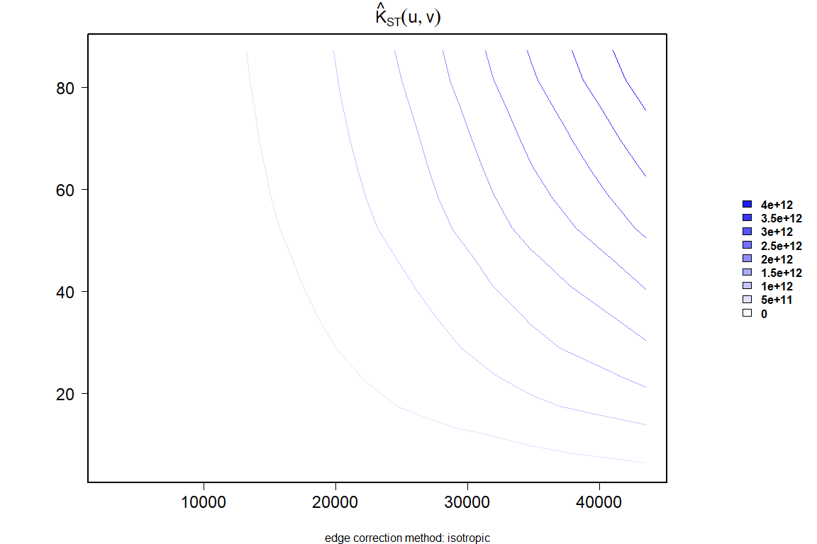
6.11.3 Guide to interpret the plot
- If the contours show high values for small values of uu and vv, it suggests clustering at short spatial and temporal distances, meaning events occur close to each other in both space and time.
- If the contours are flat or show low values, it indicates a more random distribution or a lack of significant clustering at those distances.
The spatial and temporal extent of clustering can be understood by observing how rapidly the contours increase or decrease as we move along the axes. In the plot above, we can see clustering at specific distances by observing the spacing and values of the contour lines.
6.12 Reference
Peter Hall (1990) “Using the Bootstrap to Estimate Mean Squared Error and Select Smoothing Parameter in Nonparametric Problems”, JOURNAL OF MULTIVARIATE ANALYSIS, Vol. 32, pp. 177-203.