5 2nd Order Spatial Point Patterns Analysis Methods

Published

January 23, 2023

Modified

September 6, 2025

5.1 Overview

Second-order spatial point pattern analysis examines the spatial relationships between points in a pattern, specifically focusing on how the presence of one point influences the location of others. It goes beyond simply describing the overall density of points (first-order effects) by investigating clustering, dispersion, or randomness at various spatial scales.

Using appropriate functions of spatstat, this hands-on exercise aims to discover the spatial point processes of childecare centres in Singapore.

The specific questions we would like to answer are as follows:

are the childcare centres in Singapore randomly distributed throughout the country?
if the answer is not, then the next logical question is where are the locations with higher concentration of childcare centres?

5.2 The data

To provide answers to the questions above, two data sets will be used. They are:

Child Care Services data from data.gov.sg, a point feature data providing both location and attribute information of childcare centres.
Master Plan 2019 Subzone Boundary (No Sea), a polygon feature data providing information of URA 2019 Master Plan Planning Subzone boundary data.

Both data sets are available at Singapore’s open data portal. They are provided in kml and geojson format. Students are free to download their preferred data format.

5.3 Installing and Loading the R packages

In this hands-on exercise, three R packages will be used, they are:

sf, a relatively new R package specially designed to import, manage and process vector-based geospatial data in R.
spatstat, which has a wide range of useful functions for point pattern analysis. In this hands-on exercise, it will be used to perform 1st- and 2nd-order spatial point patterns analysis and derive kernel density estimation (KDE) layer.
tmap which provides functions for plotting cartographic quality static point patterns maps or interactive maps by using leaflet API.
tidyverse, a family of R packages designed for modern data science. These packages are developed to work together seamlessly, sharing a common design philosophy, grammar, and data structures, which aims to make data manipulation, analysis, and visualization in R more intuitive and efficient.

Use the code chunk below to install and launch the five R packages.

pacman::p_load(sf, spatstat, tmap, tidyverse)

5.4 Data Import and Preparation

The processes of importing and preparing the geospatial data to meet the analysis are similar to Chapter 4. Please refer to the following sub-sections, if necessary:

Importing and Wrangling Geospatial Data Sets
Geospatial Data wrangling for preparing geospatial data in ppp object class required by spatstat package.

5.5 Second-order Spatial Point Patterns Analysis

5.6 Analysing Spatial Point Process Using G-Function

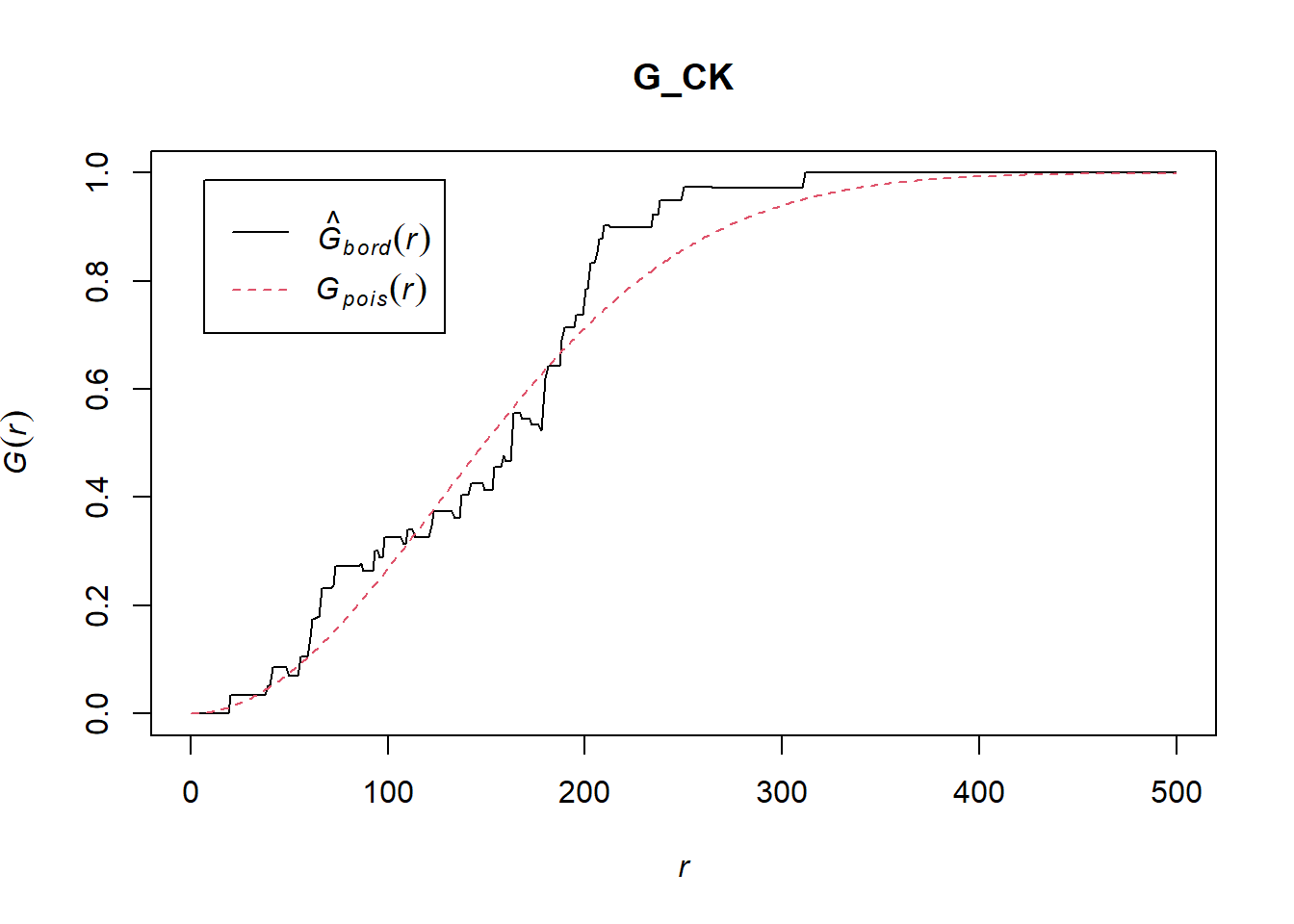
The G function measures the distribution of the distances from an arbitrary event to its nearest event. In this section, you will learn how to compute G-function estimation by using Gest() of spatstat package. You will also learn how to perform monta carlo simulation test using envelope() of spatstat package.

5.6.1 Choa Chu Kang planning area

5.6.1.1 Computing G-function estimation

set.seed(1234)

The code chunk below is used to compute G-function using Gest() of spatat package.

G_CK = Gest(childcare_ck_ppp, correction = "border")
plot(G_CK, xlim=c(0,500))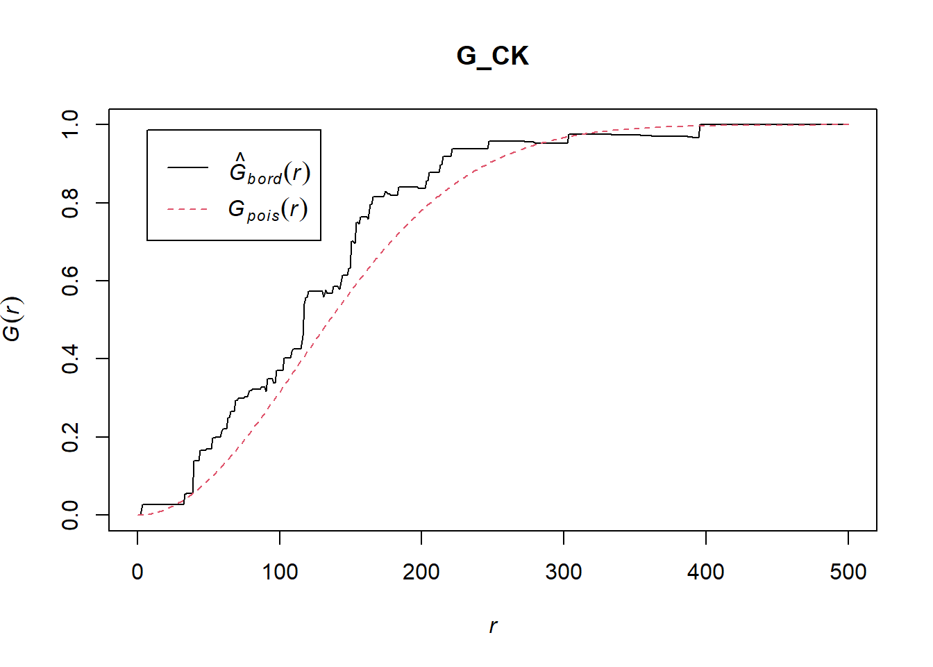

5.6.1.2 Performing Complete Spatial Randomness Test

To confirm the observed spatial patterns above, a hypothesis test will be conducted. The hypothesis and test are as follows:

Ho = The distribution of childcare services at Choa Chu Kang are randomly distributed.

H1= The distribution of childcare services at Choa Chu Kang are not randomly distributed.

The null hypothesis will be rejected if p-value is smaller than alpha value of 0.001.

Monte Carlo test with G-fucntion

G_CK.csr <- envelope(childcare_ck_ppp, Gest, nsim = 999)

Generating 999 simulations of CSR  ...
1, 2, 3, ......10.........20.........30.........40.........50.........60..
.......70.........80.........90.........100.........110.........120.........130
.........140.........150.........160.........170.........180.........190........
.200.........210.........220.........230.........240.........250.........260......
...270.........280.........290.........300.........310.........320.........330....
.....340.........350.........360.........370.........380.........390.........400..
.......410.........420.........430.........440.........450.........460.........470
.........480.........490.........500.........510.........520.........530........
.540.........550.........560.........570.........580.........590.........600......
...610.........620.........630.........640.........650.........660.........670....
.....680.........690.........700.........710.........720.........730.........740..
.......750.........760.........770.........780.........790.........800.........810
.........820.........830.........840.........850.........860.........870........
.880.........890.........900.........910.........920.........930.........940......
...950.........960.........970.........980.........990........
999.

Done.

plot(G_CK.csr)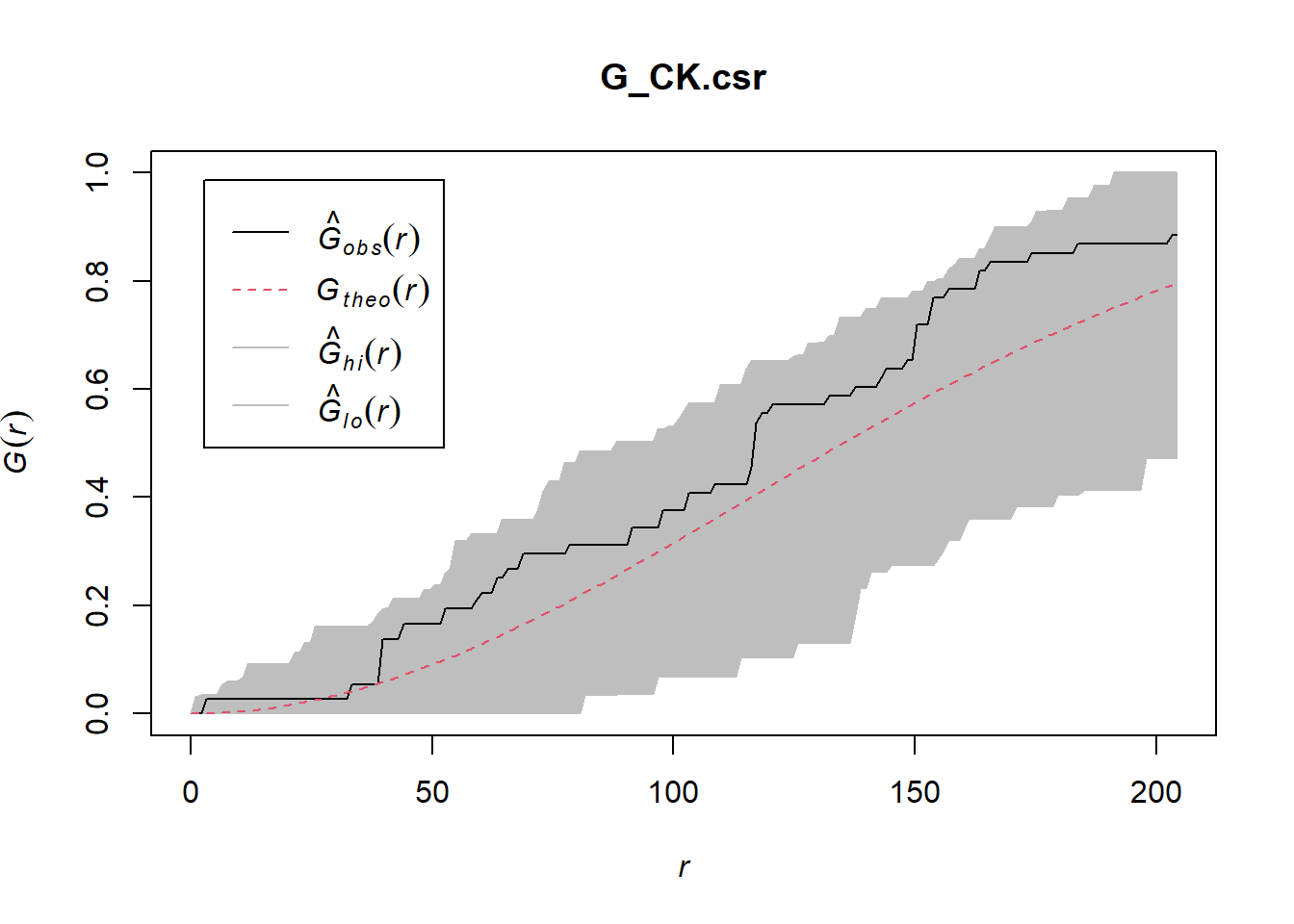

5.6.2 Tampines planning area

5.6.2.1 Computing G-function estimation

G_tm = Gest(childcare_tm_ppp, correction = "best")
plot(G_tm)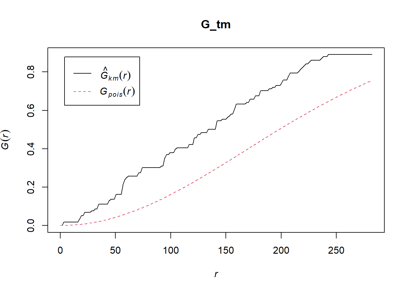

5.6.2.2 Performing Complete Spatial Randomness Test

To confirm the observed spatial patterns above, a hypothesis test will be conducted. The hypothesis and test are as follows:

Ho = The distribution of childcare services at Tampines are randomly distributed.

H1= The distribution of childcare services at Tampines are not randomly distributed.

The null hypothesis will be rejected is p-value is smaller than alpha value of 0.001.

The code chunk below is used to perform the hypothesis testing.

G_tm.csr <- envelope(childcare_tm_ppp, Gest, correction = "all", nsim = 999)

Generating 999 simulations of CSR  ...
1, 2, 3, ......10.........20.........30.........40.........50.........60..
.......70.........80.........90.........100.........110.........120.........130
.........140.........150.........160.........170.........180.........190........
.200.........210.........220.........230.........240.........250.........260......
...270.........280.........290.........300.........310.........320.........330....
.....340.........350.........360.........370.........380.........390.........400..
.......410.........420.........430.........440.........450.........460.........470
.........480.........490.........500.........510.........520.........530........
.540.........550.........560.........570.........580.........590.........600......
...610.........620.........630.........640.........650.........660.........670....
.....680.........690.........700.........710.........720.........730.........740..
.......750.........760.........770.........780.........790.........800.........810
.........820.........830.........840.........850.........860.........870........
.880.........890.........900.........910.........920.........930.........940......
...950.........960.........970.........980.........990........
999.

Done.

plot(G_tm.csr)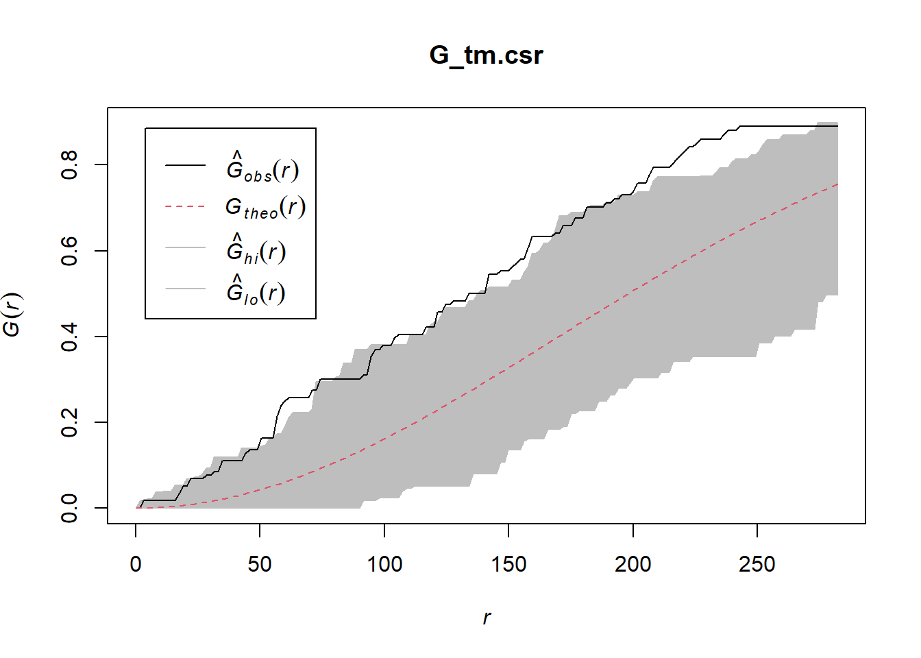

5.7 Analysing Spatial Point Process Using F-Function

The F function estimates the empty space function F(r) or its hazard rate h(r) from a point pattern in a window of arbitrary shape. In this section, you will learn how to compute F-function estimation by using Fest() of spatstat package. You will also learn how to perform monta carlo simulation test using envelope() of spatstat package.

5.7.1 Choa Chu Kang planning area

5.7.1.1 Computing F-function estimation

The code chunk below is used to compute F-function using Fest() of spatat package.

F_CK = Fest(childcare_ck_ppp)
plot(F_CK)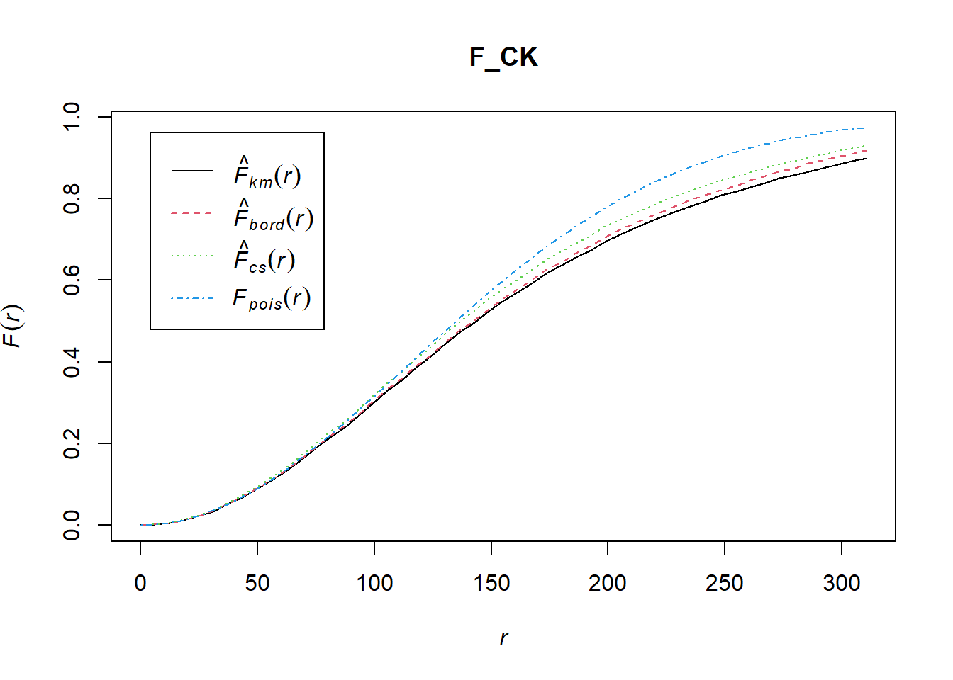

5.7.2 Performing Complete Spatial Randomness Test

To confirm the observed spatial patterns above, a hypothesis test will be conducted. The hypothesis and test are as follows:

Ho = The distribution of childcare services at Choa Chu Kang are randomly distributed.

H1= The distribution of childcare services at Choa Chu Kang are not randomly distributed.

The null hypothesis will be rejected if p-value is smaller than alpha value of 0.001.

Monte Carlo test with F-fucntion

F_CK.csr <- envelope(childcare_ck_ppp, Fest, nsim = 999)

Generating 999 simulations of CSR  ...
1, 2, 3, ......10.........20.........30.........40.........50.........60..
.......70.........80.........90.........100.........110.........120.........130
.........140.........150.........160.........170.........180.........190........
.200.........210.........220.........230.........240.........250.........260......
...270.........280.........290.........300.........310.........320.........330....
.....340.........350.........360.........370.........380.........390.........400..
.......410.........420.........430.........440.........450.........460.........470
.........480.........490.........500.........510.........520.........530........
.540.........550.........560.........570.........580.........590.........600......
...610.........620.........630.........640.........650.........660.........670....
.....680.........690.........700.........710.........720.........730.........740..
.......750.........760.........770.........780.........790.........800.........810
.........820.........830.........840.........850.........860.........870........
.880.........890.........900.........910.........920.........930.........940......
...950.........960.........970.........980.........990........
999.

Done.

plot(F_CK.csr)

5.7.3 Tampines planning area

5.7.3.1 Computing F-function estimation

Monte Carlo test with F-fucntion

F_tm = Fest(childcare_tm_ppp, correction = "best")
plot(F_tm)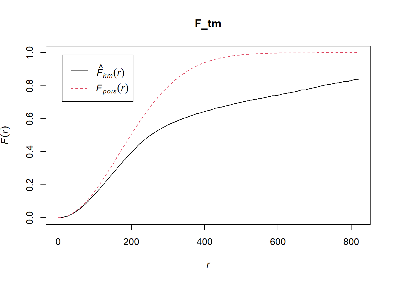

5.7.3.2 Performing Complete Spatial Randomness Test

To confirm the observed spatial patterns above, a hypothesis test will be conducted. The hypothesis and test are as follows:

Ho = The distribution of childcare services at Tampines are randomly distributed.

H1= The distribution of childcare services at Tampines are not randomly distributed.

The null hypothesis will be rejected is p-value is smaller than alpha value of 0.001.

The code chunk below is used to perform the hypothesis testing.

F_tm.csr <- envelope(childcare_tm_ppp, Fest, correction = "all", nsim = 999)

Generating 999 simulations of CSR  ...
1, 2, 3, ......10.........20.........30.........40.........50.........60..
.......70.........80.........90.........100.........110.........120.........130
.........140.........150.........160.........170.........180.........190........
.200.........210.........220.........230.........240.........250.........260......
...270.........280.........290.........300.........310.........320.........330....
.....340.........350.........360.........370.........380.........390.........400..
.......410.........420.........430.........440.........450.........460.........470
.........480.........490.........500.........510.........520.........530........
.540.........550.........560.........570.........580.........590.........600......
...610.........620.........630.........640.........650.........660.........670....
.....680.........690.........700.........710.........720.........730.........740..
.......750.........760.........770.........780.........790.........800.........810
.........820.........830.........840.........850.........860.........870........
.880.........890.........900.........910.........920.........930.........940......
...950.........960.........970.........980.........990........
999.

Done.

plot(F_tm.csr)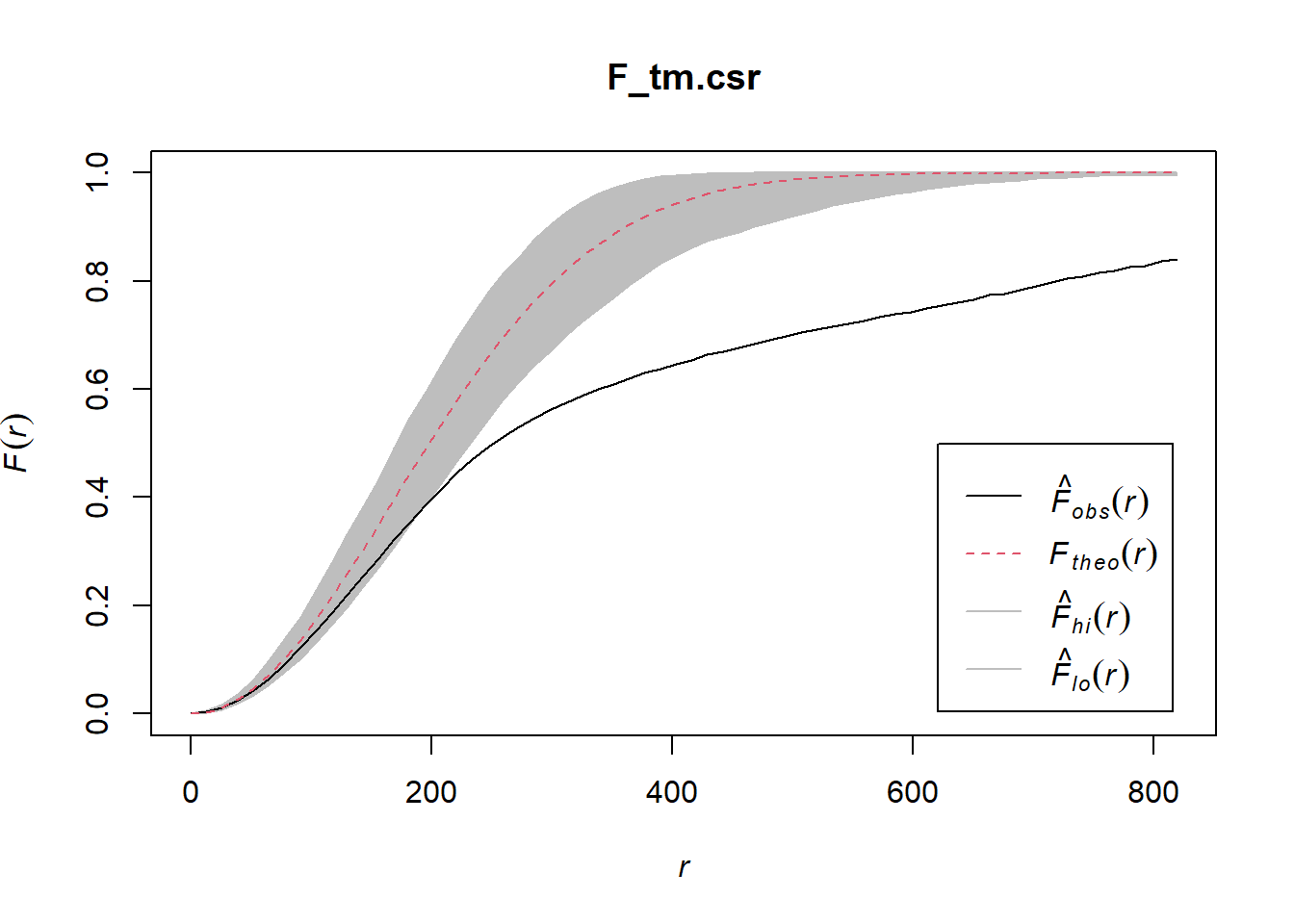

5.8 Analysing Spatial Point Process Using K-Function

K-function measures the number of events found up to a given distance of any particular event. In this section, you will learn how to compute K-function estimates by using Kest() of spatstat package. You will also learn how to perform monta carlo simulation test using envelope() of spatstat package.

5.8.1 Choa Chu Kang planning area

5.8.1.1 Computing K-fucntion estimate

K_ck = Kest(childcare_ck_ppp, correction = "Ripley")
plot(K_ck, . -r ~ r, ylab= "K(d)-r", xlab = "d(m)")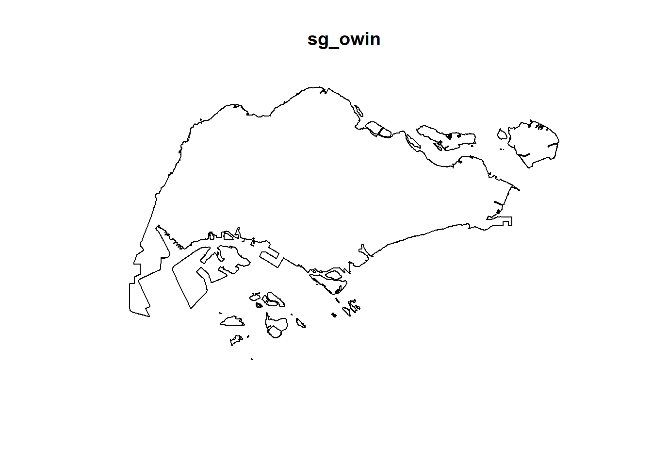

5.8.1.2 Performing Complete Spatial Randomness Test

To confirm the observed spatial patterns above, a hypothesis test will be conducted. The hypothesis and test are as follows:

Ho = The distribution of childcare services at Choa Chu Kang are randomly distributed.

H1= The distribution of childcare services at Choa Chu Kang are not randomly distributed.

The null hypothesis will be rejected if p-value is smaller than alpha value of 0.001.

The code chunk below is used to perform the hypothesis testing.

K_ck.csr <- envelope(childcare_ck_ppp, Kest, nsim = 99, rank = 1, glocal=TRUE)

Generating 99 simulations of CSR  ...
1, 2, 3, 4, 5, 6, 7, 8, 9, 10, 11, 12, 13, 14, 15, 16, 17, 18, 19, 20,
21, 22, 23, 24, 25, 26, 27, 28, 29, 30, 31, 32, 33, 34, 35, 36, 37, 38, 39, 40,
41, 42, 43, 44, 45, 46, 47, 48, 49, 50, 51, 52, 53, 54, 55, 56, 57, 58, 59, 60,
61, 62, 63, 64, 65, 66, 67, 68, 69, 70, 71, 72, 73, 74, 75, 76, 77, 78, 79, 80,
81, 82, 83, 84, 85, 86, 87, 88, 89, 90, 91, 92, 93, 94, 95, 96, 97, 98, 
99.

Done.

plot(K_ck.csr, . - r ~ r, xlab="d", ylab="K(d)-r")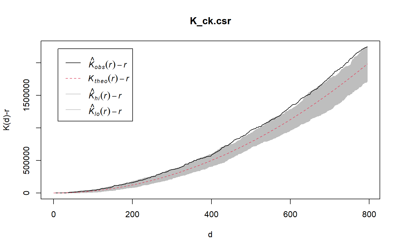

5.8.2 Tampines planning area

5.8.2.1 Computing K-fucntion estimation

K_tm = Kest(childcare_tm_ppp, correction = "Ripley")
plot(K_tm, . -r ~ r, 
     ylab= "K(d)-r", xlab = "d(m)", 
     xlim=c(0,1000))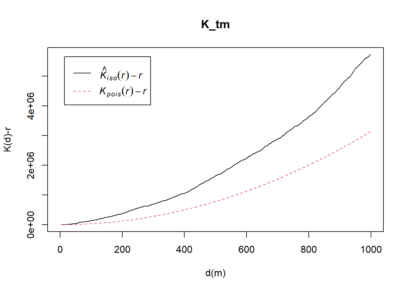

5.8.2.2 Performing Complete Spatial Randomness Test

To confirm the observed spatial patterns above, a hypothesis test will be conducted. The hypothesis and test are as follows:

Ho = The distribution of childcare services at Tampines are randomly distributed.

H1= The distribution of childcare services at Tampines are not randomly distributed.

The null hypothesis will be rejected if p-value is smaller than alpha value of 0.001.

The code chunk below is used to perform the hypothesis testing.

K_tm.csr <- envelope(childcare_tm_ppp, Kest, nsim = 99, rank = 1, glocal=TRUE)

Generating 99 simulations of CSR  ...
1, 2, 3, 4, 5, 6, 7, 8, 9, 10, 11, 12, 13, 14, 15, 16, 17, 18, 19, 20,
21, 22, 23, 24, 25, 26, 27, 28, 29, 30, 31, 32, 33, 34, 35, 36, 37, 38, 39, 40,
41, 42, 43, 44, 45, 46, 47, 48, 49, 50, 51, 52, 53, 54, 55, 56, 57, 58, 59, 60,
61, 62, 63, 64, 65, 66, 67, 68, 69, 70, 71, 72, 73, 74, 75, 76, 77, 78, 79, 80,
81, 82, 83, 84, 85, 86, 87, 88, 89, 90, 91, 92, 93, 94, 95, 96, 97, 98, 
99.

Done.

plot(K_tm.csr, . - r ~ r, 
     xlab="d", ylab="K(d)-r", xlim=c(0,500))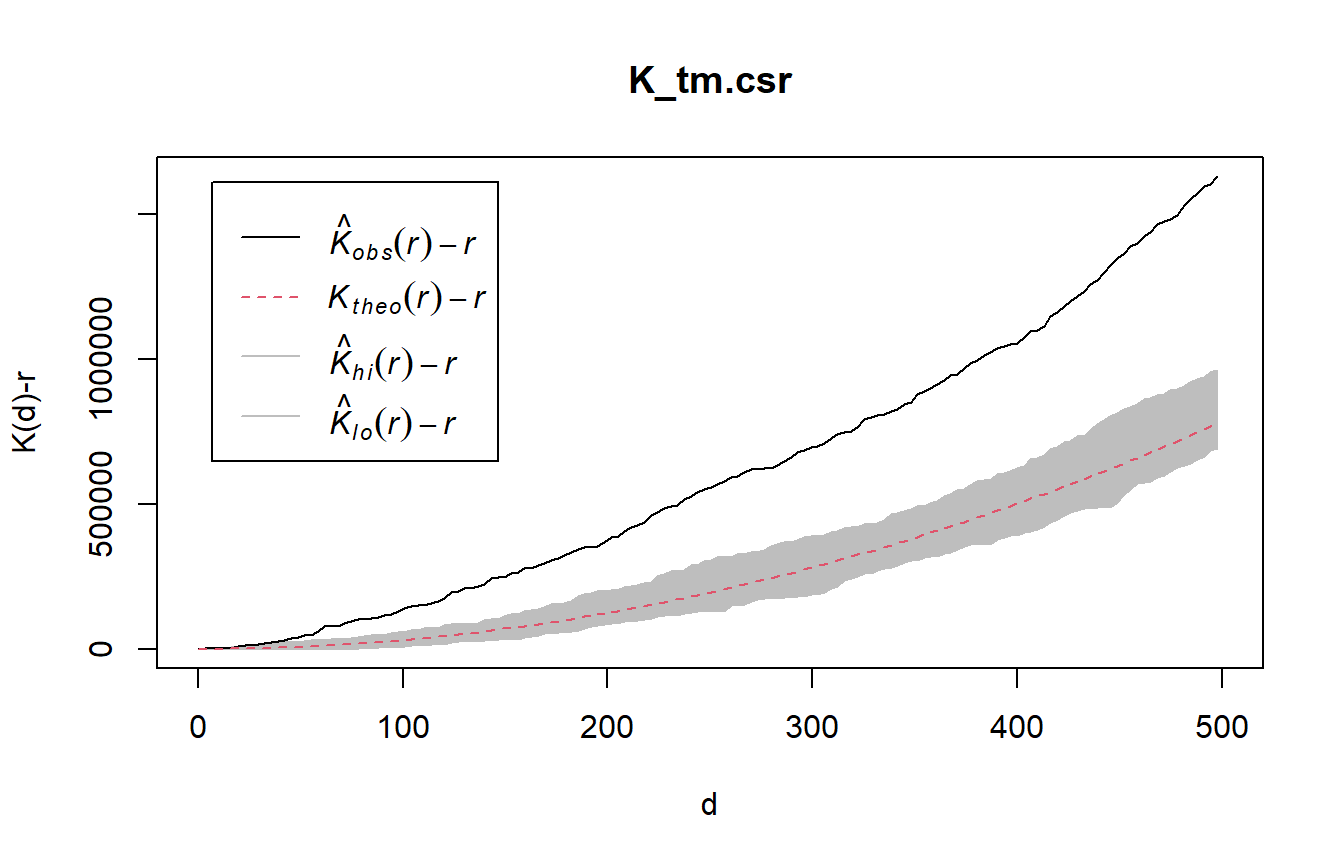

5.9 Analysing Spatial Point Process Using L-Function

In this section, you will learn how to compute L-function estimation by using Lest() of spatstat package. You will also learn how to perform monta carlo simulation test using envelope() of spatstat package.

5.9.1 Choa Chu Kang planning area

5.9.1.1 Computing L Fucntion estimation

L_ck = Lest(childcare_ck_ppp, correction = "Ripley")
plot(L_ck, . -r ~ r, 
     ylab= "L(d)-r", xlab = "d(m)")

5.9.1.2 Performing Complete Spatial Randomness Test

To confirm the observed spatial patterns above, a hypothesis test will be conducted. The hypothesis and test are as follows:

Ho = The distribution of childcare services at Choa Chu Kang are randomly distributed.

H1= The distribution of childcare services at Choa Chu Kang are not randomly distributed.

The null hypothesis will be rejected if p-value if smaller than alpha value of 0.001.

The code chunk below is used to perform the hypothesis testing.

L_ck.csr <- envelope(childcare_ck_ppp, Lest, nsim = 99, rank = 1, glocal=TRUE)

Generating 99 simulations of CSR  ...
1, 2, 3, 4, 5, 6, 7, 8, 9, 10, 11, 12, 13, 14, 15, 16, 17, 18, 19, 20,
21, 22, 23, 24, 25, 26, 27, 28, 29, 30, 31, 32, 33, 34, 35, 36, 37, 38, 39, 40,
41, 42, 43, 44, 45, 46, 47, 48, 49, 50, 51, 52, 53, 54, 55, 56, 57, 58, 59, 60,
61, 62, 63, 64, 65, 66, 67, 68, 69, 70, 71, 72, 73, 74, 75, 76, 77, 78, 79, 80,
81, 82, 83, 84, 85, 86, 87, 88, 89, 90, 91, 92, 93, 94, 95, 96, 97, 98, 
99.

Done.

plot(L_ck.csr, . - r ~ r, xlab="d", ylab="L(d)-r")

5.9.2 Tampines planning area

5.9.2.1 Computing L-fucntion estimate

L_tm = Lest(childcare_tm_ppp, correction = "Ripley")
plot(L_tm, . -r ~ r, 
     ylab= "L(d)-r", xlab = "d(m)", 
     xlim=c(0,1000))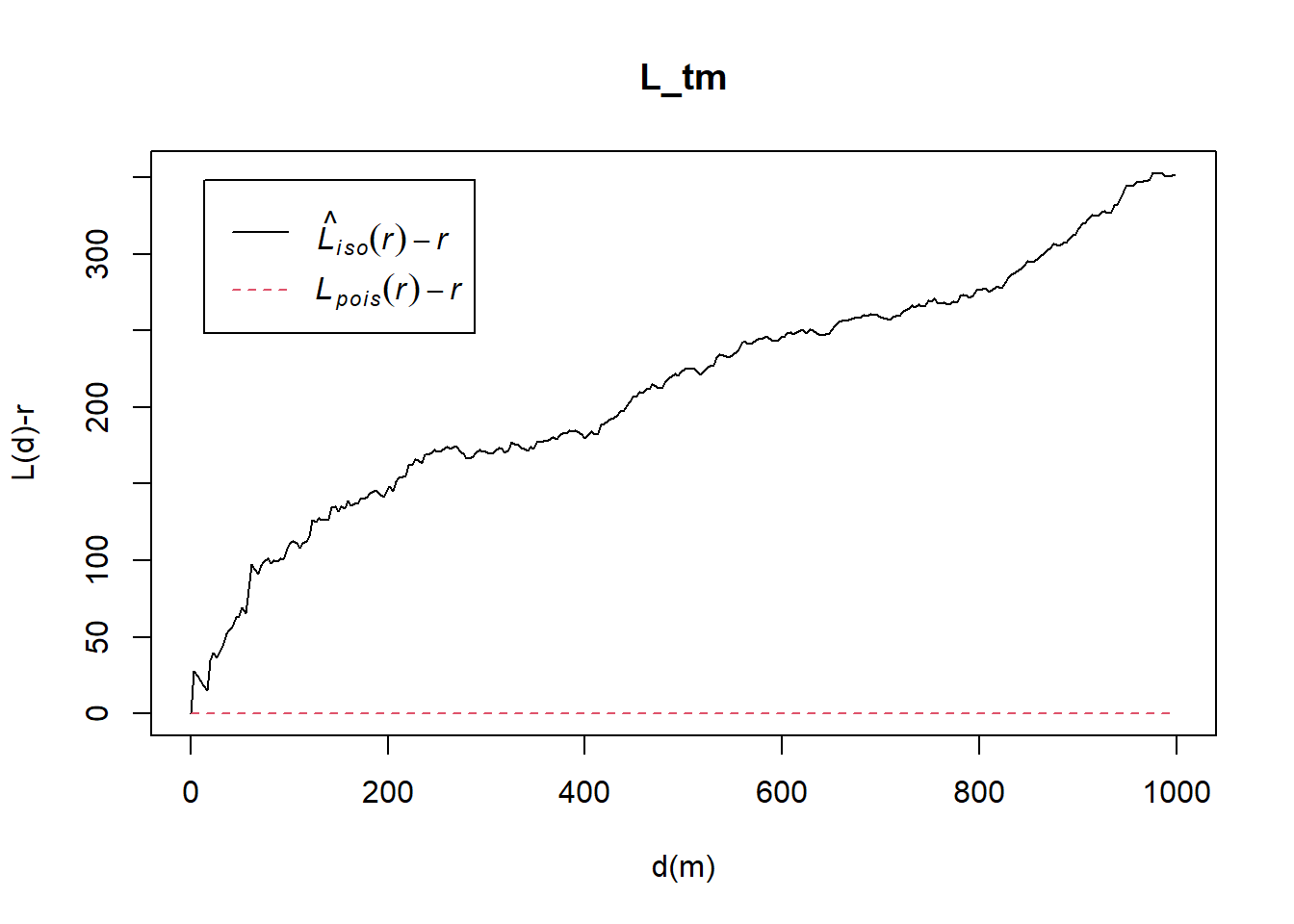

5.9.2.2 Performing Complete Spatial Randomness Test

To confirm the observed spatial patterns above, a hypothesis test will be conducted. The hypothesis and test are as follows:

Ho = The distribution of childcare services at Tampines are randomly distributed.

H1= The distribution of childcare services at Tampines are not randomly distributed.

The null hypothesis will be rejected if p-value is smaller than alpha value of 0.001.

The code chunk below will be used to perform the hypothesis testing.

L_tm.csr <- envelope(childcare_tm_ppp, Lest, nsim = 99, rank = 1, glocal=TRUE)

Generating 99 simulations of CSR  ...
1, 2, 3, 4, 5, 6, 7, 8, 9, 10, 11, 12, 13, 14, 15, 16, 17, 18, 19, 20,
21, 22, 23, 24, 25, 26, 27, 28, 29, 30, 31, 32, 33, 34, 35, 36, 37, 38, 39, 40,
41, 42, 43, 44, 45, 46, 47, 48, 49, 50, 51, 52, 53, 54, 55, 56, 57, 58, 59, 60,
61, 62, 63, 64, 65, 66, 67, 68, 69, 70, 71, 72, 73, 74, 75, 76, 77, 78, 79, 80,
81, 82, 83, 84, 85, 86, 87, 88, 89, 90, 91, 92, 93, 94, 95, 96, 97, 98, 
99.

Done.

Then, plot the model output by using the code chun below.

plot(L_tm.csr, . - r ~ r, 
     xlab="d", ylab="L(d)-r", xlim=c(0,500))